Mastering MongoDB 4.x
Second Edition
Expert techniques to run high-volume and fault-tolerant database solutions using MongoDB 4.x
Alex Giamas

BIRMINGHAM - MUMBAI
Copyright © 2019 Packt Publishing
All rights reserved. No part of this book may be reproduced, stored in a retrieval system, or transmitted in any form or by any means, without the prior written permission of the publisher, except in the case of brief quotations embedded in critical articles or reviews.
Every effort has been made in the preparation of this book to ensure the accuracy of the information presented. However, the information contained in this book is sold without warranty, either express or implied. Neither the author, nor Packt Publishing or its dealers and distributors, will be held liable for any damages caused or alleged to have been caused directly or indirectly by this book.
Packt Publishing has endeavored to provide trademark information about all of the companies and products mentioned in this book by the appropriate use of capitals. However, Packt Publishing cannot guarantee the accuracy of this information.
Commissioning Editor: Amey Varangaonkar
Acquisition Editor: Porous Godhaa
Content Development Editor: Ronnel Mathew
Technical Editor: Suwarna Patil
Copy Editor: Safis Editing
Project Coordinator: Namrata Swetta
Proofreader: Safis Editing
Indexer: Rekha Nair
Graphics: Tom Scaria
Production Coordinator: Deepika Naik
First published: November 2017
Second edition: March 2019
Production reference: 1290319
Published by Packt Publishing Ltd.
Livery Place
35 Livery Street
Birmingham
B3 2PB, UK.
ISBN 978-1-78961-787-0

Mapt is an online digital library that gives you full access to over 5,000 books and videos, as well as industry leading tools to help you plan your personal development and advance your career. For more information, please visit our website.
Spend less time learning and more time coding with practical eBooks and Videos from over 4,000 industry professionals
Improve your learning with Skill Plans built especially for you
Get a free eBook or video every month
Mapt is fully searchable
Copy and paste, print, and bookmark content
Did you know that Packt offers eBook versions of every book published, with PDF and ePub files available? You can upgrade to the eBook version at www.packt.com and as a print book customer, you are entitled to a discount on the eBook copy. Get in touch with us at customercare@packtpub.com for more details.
At www.packt.com, you can also read a collection of free technical articles, sign up for a range of free newsletters, and receive exclusive discounts and offers on Packt books and eBooks.
Alex Giamas is a consultant and a hands-on technical architect at the Department for International Trade in the UK Government. His experience spans software architecture and development using NoSQL and big data technologies. For more than 15 years, he has contributed to Fortune 15 companies and has worked as a start-up CTO.
He is the author of Mastering MongoDB 3.x, published by Packt Publishing, which is based on his use of MongoDB since 2009.
Alex has worked with a wide array of NoSQL and big data technologies, building scalable and highly available distributed software systems in Python, Java, and Ruby. He is a MongoDB Certified Developer, a Cloudera Certified Developer for Apache Hadoop and Data Science Essentials.
Doug Bierer wrote his first program on a Digital Equipment Corporation PDP-8 in 1971. Since that time, he's written buckets of code in lots of different programming languages, including BASIC, C, Assembler, PL/I, FORTRAN, Prolog, FORTH, Java, PHP, Perl, and Python. He did networking for 10 years. The largest network he worked on was based in Brussels and had 35,000 nodes. Doug is certified in PHP 5.1, 5.3, 5.5, and 7.1, and Zend Framework 1 and 2. He has authored a bunch of books and videos for O'Reilly/Packt Publishing on PHP, security, and MongoDB. His most current authoring project is a book called Learn MongoDB 4.0, scheduled to be published by Packt Publishing in September 2019. He founded unlikelysource(dot)com in April 2008.
Sumit Sengupta has worked on several RDBMS and NoSQL databases, such as Oracle, SQL Server, Postgres, MongoDB, and Cassandra. A former employee of MongoDB, he has designed, architected, and managed many distributed and big data solutions, both on-premise and on AWS and Azure. Currently, he works on the Azure Data and AI Platform for Microsoft, helping partners to create innovative solutions based on data.
If you're interested in becoming an author for Packt, please visit authors.packtpub.com and apply today. We have worked with thousands of developers and tech professionals, just like you, to help them share their insight with the global tech community. You can make a general application, apply for a specific hot topic that we are recruiting an author for, or submit your own idea.
MongoDB has grown to become the de facto NoSQL database with millions of users, from small start-ups to Fortune 500 companies. Addressing the limitations of SQL schema-based databases, MongoDB pioneered a shift of focus for DevOps and offered sharding and replication that can be maintained by DevOps teams. This book is based on MongoDB 4.0 and covers topics ranging from database querying using the shell, built-in drivers, and popular ODM mappers, to more advanced topics such as sharding, high availability, and integration with big data sources.
You will get an overview of MongoDB and will learn how to play to its strengths, with relevant use cases. After that, you will learn how to query MongoDB effectively and make use of indexes as much as possible. The next part deals with the administration of MongoDB installations, whether on-premises or on the cloud. We deal with database internals in the following section, explaining storage systems and how they can affect performance. The last section of this book deals with replication and MongoDB scaling, along with integration with heterogeneous data sources. By the end this book, you will be equipped with all the required industry skills and knowledge to become a certified MongoDB developer and administrator.
Mastering MongoDB 4.0 is a book for database developers, architects, and administrators who want to learn how to use MongoDB more effectively and productively. If you have experience with, and are interested in working with, NoSQL databases to build apps and websites, then this book is for you.
Chapter 1, MongoDB – A Database for Modern Web, takes us on a journey through web, SQL, and NoSQL technologies, from their inception to their current states.
Chapter 2, Schema Design and Data Modeling, teaches you schema design for relational databases and MongoDB, and how we can achieve the same goal from a different starting point.
Chapter 3, MongoDB CRUD Operations, provides a bird's-eye view of CRUD operations.
Chapter 4, Advanced Querying, covers advanced querying concepts using Ruby, Python, and PHP, using both the official drivers and an ODM.
Chapter 5, Multi-Document ACID Transactions, explores transactions following ACID characteristics, which is a new functionality introduced in MongoDB 4.0.
Chapter 6, Aggregation, dives deep into the aggregation framework. We also discuss when and why we should use aggregation, as opposed to MapReduce and querying the database.
Chapter 7, Indexing, explores one of the most important properties of every database, which is indexing.
Chapter 8, Monitoring, Backup, and Security, discusses the operational aspects of MongoDB. Monitoring, backup, and security should not be an afterthought, but rather are necessary processes that need to be taken care of before deploying MongoDB in a production environment.
Chapter 9, Storage Engines, teaches you about the different storage engines in MongoDB. We identify the pros and cons of each one, and the use cases for choosing each storage engine.
Chapter 10, MongoDB Tooling, covers all the different tools, both on-premises and in the cloud, that we can utilize in the MongoDB ecosystem.
Chapter 11, Harnessing Big Data with MongoDB, provides more detail on how MongoDB fits into the wider big data landscape and ecosystem.
Chapter 12, Replication, discusses replica sets and how to administer them. Starting from an architectural overview of replica sets and replica set internals around elections, we dive deep into setting up and configuring a replica set.
Chapter 13, Sharding, explores sharding, one of the most interesting features of MongoDB. We start with an architectural overview of sharding and move on to discuss how to design a shard, and especially, how to choose the right shard key.
Chapter 14, Fault Tolerance and High Availability, tries to fit in the information that we didn't manage to discuss in the previous chapters, and places emphasis on security and a series of checklists that developers and DBAs should keep into mind.
You will need the following software to be able to smoothly sail through the chapters:
You can download the example code files for this book from your account at www.packt.com. If you purchased this book elsewhere, you can visit www.packt.com/support and register to have the files emailed directly to you.
You can download the code files by following these steps:
Once the file is downloaded, please make sure that you unzip or extract the folder using the latest version of:
The code bundle for the book is also hosted on GitHub at https://github.com/PacktPublishing/Mastering-MongoDB-4.x-Second-Edition. In case there's an update to the code, it will be updated on the existing GitHub repository.
We also have other code bundles from our rich catalog of books and videos available at https://github.com/PacktPublishing/. Check them out!
In this book, you will find a number of text styles that distinguish between different kinds of information. Here are some examples of these styles and an explanation of their meaning.
Code words in text, database table names, folder names, filenames, file extensions, pathnames, dummy URLs, user input, and Twitter handles are shown as follows: "In a sharded environment, each mongod applies its own locks, thus greatly improving concurrency."
A block of code is set as follows:
db.account.find( { "balance" : { $type : 16 } } );
db.account.find( { "balance" : { $type : "integer" } } );
Any command-line input or output is written as follows:
> db.types.insert({"a":4})
WriteResult({ "nInserted" : 1 })
Bold: Indicates a new term, an important word, or words that you see onscreen. For example, words in menus or dialog boxes appear in the text like this. Here is an example: "The following screenshot shows the Zone configuration summary:"
Feedback from our readers is always welcome.
General feedback: If you have questions about any aspect of this book, mention the book title in the subject of your message and email us at customercare@packtpub.com.
Errata: Although we have taken every care to ensure the accuracy of our content, mistakes do happen. If you have found a mistake in this book, we would be grateful if you would report this to us. Please visit www.packt.com/submit-errata, selecting your book, clicking on the Errata Submission Form link, and entering the details.
Piracy: If you come across any illegal copies of our works in any form on the Internet, we would be grateful if you would provide us with the location address or website name. Please contact us at copyright@packt.com with a link to the material.
If you are interested in becoming an author: If there is a topic that you have expertise in and you are interested in either writing or contributing to a book, please visit authors.packtpub.com.
Please leave a review. Once you have read and used this book, why not leave a review on the site that you purchased it from? Potential readers can then see and use your unbiased opinion to make purchase decisions, we at Packt can understand what you think about our products, and our authors can see your feedback on their book. Thank you!
For more information about Packt, please visit packt.com.
In this section, we will go through the history of databases and how we arrived at the need for non-relational databases. We will also learn how to model our data so that storage and retrieval from MongoDB can be as efficient as possible. Even though MongoDB is schemaless, designing how data will be organized into documents can have a great effect in terms of performance.
This section consists of the following chapters:
In this chapter, we will lay the foundations for understanding MongoDB, and how it claims to be a database that's designed for the modern web. Learning in the first place is as important as knowing how to learn. We will go through the references that have the most up-to-date information about MongoDB, for both new and experienced users. We will cover the following topics:
You will require MongoDB version 4+, Apache Kafka, Apache Spark and Apache Hadoop installed to smoothly sail through the chapter. The codes that have been used for all the chapters can be found at: https://github.com/PacktPublishing/Mastering-MongoDB-4.x-Second-Edition.
Structured Query Language (SQL) existed even before the WWW. Dr. E. F. Codd originally published the paper, A Relational Model of Data for Large Shared Data Banks, in June, 1970, in the Association of Computer Machinery (ACM) journal, Communications of the ACM. SQL was initially developed at IBM by Chamberlin and Boyce, in 1974. Relational Software (now Oracle Corporation) was the first to develop a commercially available implementation of SQL, targeted at United States governmental agencies.
The first American National Standards Institute (ANSI) SQL standard came out in 1986. Since then, there have been eight revisions, with the most recent being published in 2016 (SQL:2016).
SQL was not particularly popular at the start of the WWW. Static content could just be hardcoded into the HTML page without much fuss. However, as the functionality of websites grew, webmasters wanted to generate web page content driven by offline data sources, in order to generate content that could change over time without redeploying code.
Common Gateway Interface (CGI) scripts, developing Perl or Unix shells, were driving early database-driven websites in Web 1.0. With Web 2.0, the web evolved from directly injecting SQL results into the browser to using two-tier and three-tier architectures that separated views from the business and model logic, allowing for SQL queries to be modular and isolated from the rest of the web application.
On the other hand, Not only SQL (NoSQL) is much more modern and supervened web evolution, rising at the same time as Web 2.0 technologies. The term was first coined by Carlo Strozzi in 1998, for his open source database that did not follow the SQL standard, but was still relational.
This is not what we currently expect from a NoSQL database. Johan Oskarsson, a developer at Last.fm at the time, reintroduced the term in early 2009, in order to group a set of distributed, non-relational data stores that were being developed. Many of them were based on Google's Bigtable and MapReduce papers, or Amazon's DynamoDB, a highly available key-value based storage system.
NoSQL's foundations grew upon relaxed atomicity, consistency, isolation, and durability (ACID) properties, which guarantee the performance, scalability, flexibility, and reduced complexity. Most NoSQL databases have gone one way or another in providing as many of the previously mentioned qualities as possible, even offering adjustable guarantees to the developer. The following diagram describes the evolution of SQL and NoSQL:

10gen started to develop a cloud computing stack in 2007 and soon realized that the most important innovation was centered around the document-oriented database that they built to power it, which was MongoDB. MongoDB was initially released on August 27, 2009.
Version 1 of MongoDB was pretty basic in terms of features, authorization, and ACID guarantees but it made up for these shortcomings with performance and flexibility.
In the following sections, we will highlight the major features of MongoDB, along with the version numbers with which they were introduced.
The different features of versions 1.0 and 1.2 are as follows:
The different features of version 2.0 are as follows:
The different features of version 3.0 are as follows:
The different features of version 4.0 are as follows:
The following diagram shows MongoDB's evolution:

As we can observe, version 1 was pretty basic, whereas version 2 introduced most of the features present in the current version, such as sharding, usable and special indexes, geospatial features, and memory and concurrency improvements.
On the way from version 2 to version 3, the aggregation framework was introduced, mainly as a supplement to the ageing (and never up to par with dedicated frameworks, such as Hadoop) MapReduce framework. Then, text search was added, and slowly but surely, the framework was improving performance, stability, and security, to adapt to the increasing enterprise load of customers using MongoDB.
With WiredTiger's introduction in version 3, locking became much less of an issue for MongoDB, as it was brought down from the process (global lock) to the document level, almost the most granular level possible.
Version 4 marked a major transition, bridging the SQL and NoSQL world with the introduction of multi-document ACID transactions. This allowed for a wider range of applications to use MongoDB, especially applications that require a strong real-time consistency guarantee. Further, the introduction of change streams allowed for a faster time to market for real-time applications using MongoDB. A series of tools have also been introduced, to facilitate serverless, mobile, and Internet of Things (IoT) development.
In its current state, MongoDB is a database that can handle loads ranging from start up MVPs and POCs to enterprise applications with hundreds of servers.
MongoDB was developed in the Web 2.0 era. By then, most developers had been using SQL or object-relational mapping (ORM) tools from their language of choice to access RDBMS data. As such, these developers needed an easy way to get acquainted with MongoDB from their relational background.
Thankfully, there have been several attempts at making SQL to MongoDB cheat sheets that explain the MongoDB terminology in SQL terms.
On a higher level, we have the following:
Some more examples of common operations are shown in the following table:
|
SQL |
MongoDB |
|
Database |
Database |
|
Table |
Collection |
|
Index |
Index |
|
Row |
Document |
|
Column |
Field |
|
Joins |
Embed in document or link via DBRef |
|
CREATE TABLE employee (name VARCHAR(100)) |
db.createCollection("employee") |
|
INSERT INTO employees VALUES (Alex, 36) |
db.employees.insert({name: "Alex", age: 36}) |
|
SELECT * FROM employees |
db.employees.find() |
|
SELECT * FROM employees LIMIT 1 |
db.employees.findOne() |
|
SELECT DISTINCT name FROM employees |
db.employees.distinct("name") |
|
UPDATE employees SET age = 37 WHERE name = 'Alex' |
db.employees.update({name: "Alex"}, {$set: {age: 37}}, {multi: true}) |
|
DELETE FROM employees WHERE name = 'Alex' |
db.employees.remove({name: "Alex"}) |
|
CREATE INDEX ON employees (name ASC) |
db.employees.ensureIndex({name: 1}) |
Further examples of common operations can be seen at http://s3.amazonaws.com/info-mongodb-com/sql_to_mongo.pdf.
As MongoDB has grown from being a niche database solution to the Swiss Army knife of NoSQL technologies, more developers are coming to it from a NoSQL background, as well.
Putting the SQL to NoSQL differences aside, it is users from columnar-type databases that face the most challenges. With Cassandra and HBase being the most popular column-oriented database management systems, we will examine the differences and how a developer can migrate a system to MongoDB. The different features of MongoDB for NoSQL developers are as follows:
In this section, we will analyze MongoDB's characteristics as a database. Understanding the features that MongoDB provides can help developers and architects to evaluate the requirements at hand and how MongoDB can help to fulfill them. Also, we will go over some common use cases from the experience of MongoDB, Inc. that have delivered the best results for its users.
MongoDB has grown to become a general purpose NoSQL database, offering the best of both the RDBMS and NoSQL worlds. Some of the key characteristics are as follows:
Since MongoDB is a highly popular NoSQL database, there have been several use cases where it has succeeded in supporting quality applications, with a great delivery time to the market.
Many of its most successful use cases center around the following areas:
All of these success stories share some common characteristics. We will try to break them down in order of relative importance:
MongoDB's criticism is associated with the following points:
In this section, we will present some of the best practice around operations, schema design, durability, replication, sharding, and security. Further information on when to implement these best practices will be presented in later chapters.
As a database, MongoDB is built with developers in mind, and it was developed during the web era, so it does not require as much operational overhead as traditional RDBMS. That being said, there are some best practices that need to be followed to be proactive and achieve high availability goals.
In order of importance, the best practices are as follows:
MongoDB is schema-less, and you have to design your collections and indexes to accommodate for this fact:
Writing durability can be fine-tuned in MongoDB, and, according to our application design, it should be as strict as possible, without affecting our performance goals.
Fine-tune the data and flush it to the disk interval in the WiredTiger storage engine, the default is to flush data to the disk every 60 seconds after the last checkpoint, or after 2 GB of data has been written. This can be changed by using the --wiredTigerCheckpointDelaySecs command-line option.
In MMAPv1, data files are flushed to the disk every 60 seconds. This can be changed by using the --syncDelay command-line option. We can also perform various tasks, such as the following:
Replica sets are MongoDB's mechanism to provide redundancy, high availability, and higher read throughput, under the right conditions. In MongoDB, replication is easy to configure and focus in operational terms:
Sharding is MongoDB's solution for horizontal scaling. In Chapter 8, Monitoring, Backup, and Security, we will go over its usage in more detail, but the following are some best practices, based on the underlying data architecture:
Security is always a multi-layered approach, and these few recommendations do not form an exhaustive list; they are just the bare basics that need to be done in any MongoDB database:
When we are using MongoDB, we can use our own servers in a data center, a MongoDB-hosted solution such as MongoDB Atlas, or we can get instances from Amazon by using EC2. EC2 instances are virtualized and share resources in a transparent way, with collocated VMs in the same physical host. So, there are some more considerations to take into account if you are going down that route, as follows:
Reading a book is great (and reading this book is even greater), but continuous learning is the only way to keep up to date with MongoDB. In the following sections, we will highlight the places that you should go for updates and development/operational references.
The online documentation available at https://docs.mongodb.com/manual/ is the starting point for every developer, new or seasoned.
The JIRA tracker is a great place to take a look at fixed bugs and the features that are coming up next: https://jira.mongodb.org/browse/SERVER/.
Some other great books on MongoDB are as follows:
The MongoDB user group (https://groups.google.com/forum/#!forum/mongodb-user) has a great archive of user questions about features and long-standing bugs. It is a place to go when something doesn't work as expected.
Online forums (Stack Overflow and Reddit, among others) are always a source of knowledge, with the caveat that something may have been posted a few years ago and may not apply anymore. Always check before trying.
Finally, MongoDB University is a great place to keep your skills up to date and to learn about the latest features and additions: https://university.mongodb.com/.
In this chapter, we started our journey through web, SQL, and NoSQL technologies, from their inception to their current states. We identified how MongoDB has been shaping the world of NoSQL databases over the years, and how it is positioned against other SQL and NoSQL solutions.
We explored MongoDB's key characteristics and how MongoDB has been used in production deployments. We identified the best practices for designing, deploying, and operating MongoDB.
Initially, we identified how to learn by going through documentation and online resources that can be used to stay up-to-date with the latest features and developments.
In the next chapter, we will go deeper into schema design and data modeling, looking at how to connect to MongoDB by using both the official drivers and an Object Document Mapper (ODM), a variation of object-relational mappers for NoSQL databases.
This chapter will focus on schema design for schema less databases such as MongoDB. Although this may sound counter-intuitive, there are considerations that we should take into account when we develop for MongoDB. We will learn about the schema considerations and the data types supported by MongoDB. We will also learn about preparing data for text searches in MongoDB by connecting Ruby, Python, and PHP.
In this chapter, we will cover the following topics:
In relational databases, we design with the goal of avoiding anomalies and redundancy. Anomalies can happen when we have the same information stored in multiple columns; we update one of them but not the rest and so end up with conflicting information for the same column of information. An anomaly can also happen when we cannot delete a row without losing information that we need, possibly in other rows referenced by it. Data redundancy can happen when our data is not in a normal form, but has duplicate data across different tables. This can lead to data inconsistency and is difficult to maintain.
In relational databases, we use normal forms to normalize our data. Starting from the basic First Normal Form (1NF), onto the 2NF, 3NF, and BCNF, we model our data, taking functional dependencies into account and, if we follow the rules, we can end up with many more tables than domain model objects.
In practice, relational database modeling is often driven by the structure of the data that we have. In web applications following some sort of Model-View-Controller (MVC) model pattern, we will model our database according to our models, which are modeled after the Unified Modeling Language (UML) diagram conventions. Abstractions such as the ORM for Django or the Active Record for Rails help application developers abstract database structure to object models. Ultimately, many times, we end up designing our database based on the structure of the available data. Thus, we are designing around the answers that we can have.
In contrast to relational databases, in MongoDB we have to base our modeling on our application-specific data access patterns. Finding out the questions that our users will have is paramount to designing our entities. In contrast to an RDBMS, data duplication and denormalization are used far more frequently and with solid reason.
The document model that MongoDB uses means that every document can hold substantially more or less information than the next one, even within the same collection. Coupled with rich and detailed queries being possible in MongoDB in the embedded document level, this means that we are free to design our documents in any way that we want. When we know our data access patterns, we can estimate which fields need to be embedded and which can be split out to different collections.
The read to write ratio is often an important design consideration for MongoDB modeling. When reading data, we want to avoid scatter/gather situations, where we have to hit several shards with random I/O requests to get the data our application needs.
When writing data, on the other hand, we want to spread out writes to as many servers as possible, to avoid overloading any single one of them. These goals appear to be conflicting on the surface, but they can be combined once we know our access patterns, coupled with application design considerations, such as using a replica set to read from secondary nodes.
In this section, we will discuss the different data types MongoDB uses, how they map to the data types that programming languages use, and how we can model data relationships in MongoDB using Ruby, Python, and PHP.
MongoDB uses BSON, a binary-encoded serialization for JSON documents. BSON extends the JSON data types, offering, for example, native data and binary data types.
BSON, compared to protocol buffers, allows for more flexible schemas that come at the cost of space efficiency. In general, BSON is space-efficient, easy to traverse, and time-efficient in encoding/decoding operations, as can be seen in the following table. (See the MongoDB documentation at https://docs.mongodb.com/manual/reference/bson-types/):
|
Type |
Number |
Alias |
Notes |
|
Double |
1 |
double |
|
|
String |
2 |
string |
|
|
Object |
3 |
object |
|
|
Array |
4 |
array |
|
|
Binary data |
5 |
binData |
|
|
ObjectID |
7 |
objectId |
|
|
Boolean |
8 |
bool |
|
|
Date |
9 |
date |
|
|
Null |
10 |
null |
|
|
Regular expression |
11 |
regex |
|
|
JavaScript |
13 |
javascript |
|
|
JavaScript (with scope) |
15 |
javascriptWithScope |
|
|
32-bit integer |
16 |
int |
|
|
Timestamp |
17 |
timestamp |
|
|
64-bit integer |
18 |
long |
|
|
Decimal128 |
19 |
decimal |
New in version 3.4 |
|
Min key |
-1 |
minKey |
|
|
Max key |
127 |
maxKey |
|
|
Undefined |
6 |
undefined |
Deprecated |
|
DBPointer |
12 |
dbPointer |
Deprecated |
|
Symbol |
14 |
symbol |
Deprecated |
In MongoDB, we can have documents with different value types for a given field and we distinguish among them when querying using the $type operator.
For example, if we have a balance field in GBP with 32-bit integers and double data types, if balance has pennies in it or not, we can easily query for all accounts that have a rounded balance with any of the following queries shown in the example:
db.account.find( { "balance" : { $type : 16 } } );
db.account.find( { "balance" : { $type : "integer" } } );
We will compare the different data types in the following section.
Due to the nature of MongoDB, it's perfectly acceptable to have different data type objects in the same field. This may happen by accident or on purpose (that is, null and actual values in a field).
The sorting order of different types of data, from highest to lowest, is as follows:
Non-existent fields get sorted as if they have null in the respective field. Comparing arrays is a bit more complex than fields. An ascending order of comparison (or <) will compare the smallest element of each array. A descending order of comparison (or >) will compare the largest element of each array.
For example, see the following scenario:
> db.types.find()
{ "_id" : ObjectId("5908d58455454e2de6519c49"), "a" : [ 1, 2, 3 ] }
{ "_id" : ObjectId("5908d59d55454e2de6519c4a"), "a" : [ 2, 5 ] }
In ascending order, this is as follows:
> db.types.find().sort({a:1})
{ "_id" : ObjectId("5908d58455454e2de6519c49"), "a" : [ 1, 2, 3 ] }
{ "_id" : ObjectId("5908d59d55454e2de6519c4a"), "a" : [ 2, 5 ] }
However, in descending order, it is as follows:
> db.types.find().sort({a:-1})
{ "_id" : ObjectId("5908d59d55454e2de6519c4a"), "a" : [ 2, 5 ] }
{ "_id" : ObjectId("5908d58455454e2de6519c49"), "a" : [ 1, 2, 3 ] }
The same applies when comparing an array with a single number value, as illustrated in the following example. Inserting a new document with an integer value of 4 is done as follows:
> db.types.insert({"a":4})
WriteResult({ "nInserted" : 1 })
The following example shows the code snippet for a descending sort:
> db.types.find().sort({a:-1})
{ "_id" : ObjectId("5908d59d55454e2de6519c4a"), "a" : [ 2, 5 ] }
{ "_id" : ObjectId("5908d73c55454e2de6519c4c"), "a" : 4 }
{ "_id" : ObjectId("5908d58455454e2de6519c49"), "a" : [ 1, 2, 3 ] }
And the following example is the code snippet for an ascending sort:
> db.types.find().sort({a:1})
{ "_id" : ObjectId("5908d58455454e2de6519c49"), "a" : [ 1, 2, 3 ] }
{ "_id" : ObjectId("5908d59d55454e2de6519c4a"), "a" : [ 2, 5 ] }
{ "_id" : ObjectId("5908d73c55454e2de6519c4c"), "a" : 4 }
In each case, we highlighted the values being compared in bold.
We will learn about the data type in the following section.
Dates are stored as milliseconds with effect from January 01, 1970 (epoch time). They are 64-bit signed integers, allowing for a range of 135 million years before and after 1970. A negative date value denotes a date before January 01, 1970. The BSON specification refers to the date type as UTC DateTime.
Dates in MongoDB are stored in UTC. There isn't timestamp with a timezone data type like in some relational databases. Applications that need to access and modify timestamps, based on local time, should store the timezone offset together with the date and offset dates on an application level.
In the MongoDB shell, this could be done using the following format with JavaScript:
var now = new Date();
db.page_views.save({date: now,
                    offset: now.getTimezoneOffset()});
Then you need to apply the saved offset to reconstruct the original local time, as in the following example:
var record = db.page_views.findOne();
var localNow = new Date( record.date.getTime() - ( record.offset * 60000 ) );
In the next section, we will cover ObjectId.
ObjectId is a special data type for MongoDB. Every document has an _id field from cradle to grave. It is the primary key for each document in a collection and has to be unique. If we omit this field in a create statement, it will be assigned automatically with an ObjectId.
Messing with ObjectId is not advisable but we can use it (with caution!) for our purposes.
ObjectId has the following distinctions:
The structure of an ObjectId has the following:
The following diagram shows the structure of an ObjectID:

By its structure, ObjectId will be unique for all purposes; however, since this is generated on the client side, you should check the underlying library's source code to verify that implementation is according to specification.
In the next section, we will learn about modeling data for atomic operations.
MongoDB is relaxing many of the typical Atomicity, Consistency, Isolation and Durability (ACID) constraints found in RDBMS. In the absence of transactions, it can sometimes be difficult to keep the state consistent across operations, especially in the event of failures.
Luckily, some operations are atomic at the document level:
These are all atomic (all or nothing) for a single document.
This means that, if we embed information in the same document, we can make sure they are always in sync.
An example would be an inventory application, with a document per item in our inventory, where we would need to total the available items left in stock how many have been placed in a shopping cart in sync, and use this data to sum up the total available items.
With total_available = 5, available_now = 3, shopping_cart_count = 2, this use case could look like the following: {available_now : 3, Shopping_cart_by: ["userA", "userB"] }
When someone places the item in their shopping cart, we can issue an atomic update, adding their user ID in the shopping_cart_by field and, at the same time, decreasing the available_now field by one.
This operation will be guaranteed to be atomic at the document level. If we need to update multiple documents within the same collection, the update operation may complete successfully without modifying all of the documents that we intended it to. This could happen because the operation is not guaranteed to be atomic across multiple document updates.
This pattern can help in some, but not all, cases. In many cases, we need multiple updates to be applied on all or nothing across documents, or even collections.
A typical example would be a bank transfer between two accounts. We want to subtract x GBP from user A, then add x to user B. If we fail to do either of the two steps, we would return to the original state for both balances.
The details of this pattern are outside the scope of this book, but roughly, the idea is to implement a hand-coded two phase commit protocol. This protocol should create a new transaction entry for each transfer with every possible state in this transaction: such as initial, pending, applied, done, cancelling, cancelled, and, based on the state that each transaction is left at, applying the appropriate rollback function to it.
If you find yourself having to implement transactions in a database that was built to avoid them, take a step back and rethink why you need to do that.
Sparingly, we could use $isolated to isolate writes to multiple documents from other writers or readers to these documents. In the previous example, we could use $isolated to update multiple documents and make sure that we update both balances before anyone else gets the chance to double-spend, draining the source account of its funds.
What this won't give us though, is atomicity, the all-or-nothing approach. So, if the update only partially modifies both accounts, we still need to detect and unroll any modifications made in the pending state.
$isolated uses an exclusive lock on the entire collection, no matter which storage engine is used. This means a severe speed penalty when using it, especially for WiredTiger document-level locking semantics.
$isolated does not work with sharded clusters, which may be an issue when we decide to go from replica sets to sharded deployment.
MongoDB read operations would be characterized as read uncommitted in a traditional RDBMS definition. What this means is that, by default, reads may get values that may not finally persist to the disk in the event of, for example, data loss or a replica set rollback operation.
In particular, when updating multiple documents with the default write behavior, lack of isolation may result in the following:
These can be resolved by using the $isolated operator with a heavy performance penalty.
Queries with cursors that don't use .snapshot() may also, in some cases, get inconsistent results. This can happen if the query's resultant cursor fetches a document, which receives an update while the query is still fetching results, and, because of insufficient padding, ends up in a different physical location on the disk, ahead of the query's result cursor position. .snapshot() is a solution for this edge case, with the following limitations:
If our collection has mostly static data, we can use a unique index in the query field to simulate snapshot() and still be able to apply sort() to it.
All in all, we need to apply safeguards at the application level to make sure that we won't end up with unexpected results.
Starting from version 3.4, MongoDB offers linearizable read concern. With linearizable read concern from the primary member of a replica set and a majority write concern, we can ensure that multiple threads can read and write a single document as if a single thread was performing these operations one after the other. This is considered a linearizable schedule in RDBMS, and MongoDB calls it the real-time order.
In the following sections, we will explain how we can translate relationships in RDBMS theory into MongoDB's document-collection hierarchy. We will also examine how we can model our data for text search in MongoDB.
Coming from the relational DB world, we identify objects by their relationships. A one-to-one relationship could be a person with an address. Modeling it in a relational database would most probably require two tables: a Person and an Address table with a foreign key person_id in the Address table, as shown in the following diagram:

The perfect analogy in MongoDB would be two collections, Person and Address, as shown in the following code:
> db.Person.findOne()
{
"_id" : ObjectId("590a530e3e37d79acac26a41"), "name" : "alex"
}
> db.Address.findOne()
{
"_id" : ObjectId("590a537f3e37d79acac26a42"),
"person_id" : ObjectId("590a530e3e37d79acac26a41"),
"address" : "N29DD"
}
Now, we can use the same pattern as we do in a relational database to find Person from address, as shown in the following example:
> db.Person.find({"_id": db.Address.findOne({"address":"N29DD"}).person_id})
{
"_id" : ObjectId("590a530e3e37d79acac26a41"), "name" : "alex"
}
This pattern is well known and works in the relational world.
In MongoDB, we don't have to follow this pattern, as there are more suitable ways to model these kinds of relationship.
One way in which we would typically model one-to-one or one-to-many relationships in MongoDB would be through embedding. If the person has two addresses, then the same example would then be shown in the following way:
{ "_id" : ObjectId("590a55863e37d79acac26a43"), "name" : "alex", "address" : [ "N29DD", "SW1E5ND" ] }
Using an embedded array, we can have access to every address this user has. Embedding querying is rich and flexible so that we can store more information in each document, as shown in the following example:
{ "_id" : ObjectId("590a56743e37d79acac26a44"),
"name" : "alex",
"address" : [ { "description" : "home", "postcode" : "N29DD" },
{ "description" : "work", "postcode" : "SW1E5ND" } ] }
The advantages of this approach are as follows:
The most notable disadvantage is that the maximum size of the document is 16 MB so this approach cannot be used for an arbitrary, ever-growing number of attributes. Storing hundreds of elements in embedded arrays will also degrade performance.
When the number of elements in the many side of the relationship can grow unbounded, it's better to use references. References can come in two forms:
> db.Person.findOne()
{ "_id" : ObjectId("590a530e3e37d79acac26a41"), "name" : "alex", addresses:
[ ObjectID('590a56743e37d79acac26a44'),
ObjectID('590a56743e37d79acac26a46'),
ObjectID('590a56743e37d79acac26a54') ] }
> person = db.Person.findOne({"name":"mary"})
> addresses = db.Addresses.find({_id: {$in: person.addresses} })
Turning this one-to-many to many-to-many is as easy as storing this array in both ends of the relationship (that is, in the Person and Address collections).
> db.Address.find()
{ "_id" : ObjectId("590a55863e37d79acac26a44"), "person":  ObjectId("590a530e3e37d79acac26a41"), "address" : [ "N29DD" ] }
{ "_id" : ObjectId("590a55863e37d79acac26a46"), "person":  ObjectId("590a530e3e37d79acac26a41"), "address" : [ "SW1E5ND" ] }
{ "_id" : ObjectId("590a55863e37d79acac26a54"), "person":  ObjectId("590a530e3e37d79acac26a41"), "address" : [ "N225QG" ] }
> person = db.Person.findOne({"name":"alex"})
> addresses = db.Addresses.find({"person": person._id})
As we can see, with both designs we need to make two queries to the database to fetch the information. The second approach has the advantage that it won't let any document grow unbounded, so it can be used in cases where one-to-many is one-to-millions.
Searching for keywords in a document is a common operation for many applications. If this is a core operation, it makes sense to use a specialized store for search, such as Elasticsearch; however, MongoDB can be used efficiently until scale dictates moving to a different solution.
The basic need for a keyword search is to be able to search the entire document for keywords. For example, with a document in the products collection, as shown in the following code:
{ name : "Macbook Pro late 2016 15in" ,
  manufacturer : "Apple" ,
  price: 2000 ,
  keywords : [ "Macbook Pro late 2016 15in", "2000", "Apple", "macbook", "laptop", "computer" ]
 }
We can create a multi-key index in the keywords field, as shown in the following code:
> db.products.createIndex( { keywords: 1 } )
Now we can search in the keywords field for any name, manufacturer, price, and also any of the custom keywords that we set up. This is not an efficient or flexible approach, as we need to keep keywords lists in sync, we can't use stemming, and we can't rank results (it's more like filtering than searching). The only advantage of this method is that it is slightly quicker to implement.
Since version 2.4, MongoDB has had a special text index type. This can be declared in one or multiple fields and supports stemming, tokenization, exact phrase (" "), negation (-), and weighting results.
Index declaration on three fields with custom weights is shown in the following example:
db.products.createIndex({
     name: "text",
     manufacturer: "text",
    price: "text"
   },
  {
     weights: { name: 10,
       manufacturer: 5,
      price: 1 },
     name: "ProductIndex"
   })
In this example, name is 10 times more important than price but only two times from manufacturer.
A text index can also be declared with a wildcard, matching all the fields that match the pattern, as shown in the following example:
db.collection.createIndex( { "$**": "text" } )
This can be useful when we have unstructured data and we may not know all the fields that they will come with. We can drop the index by name, just like with any other index.
The greatest advantage though, other than all the features, is that all record keeping is done by the database.
In the next section, we will learn how to connect to MongoDB.
There are two ways to connect to MongoDB. The first is by using the driver for your programming language. The second is by using an ODM layer to map your model objects to MongoDB in a transparent way. In this section, we will cover both ways, using three of the most popular languages for web application development: Ruby, Python, and PHP.
Ruby was one of the first languages to have support from MongoDB with an official driver. The official MongoDB Ruby driver on GitHub is the recommended way to connect to a MongoDB instance. Perform the following steps to connect MongoDB using Ruby:
gem 'mongo', '~> 2.6'
require 'mongo'
client = Mongo::Client.new([ '127.0.0.1:27017' ], database: 'test')
client_host = ['server1_hostname:server1_ip, server2_hostname:server2_ip']
 client_options = {
  database: 'YOUR_DATABASE_NAME',
  replica_set: 'REPLICA_SET_NAME',
  user: 'YOUR_USERNAME',
  password: 'YOUR_PASSWORD'
 }
client = Mongo::Client.new(client_host, client_options)
Using a low-level driver to connect to the MongoDB database is often not the most efficient route. All the flexibility that a low-level driver provides is offset against longer development times and code to glue our models with the database.
An ODM can be the answer to these problems. Just like ORMs, ODMs bridge the gap between our models and the database. In Rails, the most widely-used MVC framework for Ruby—Mongoid—can be used to model our data in a similar way to Active Record.
Installing gem is similar to the Mongo Ruby driver, by adding a single file in the Gemfile, as shown in the following code:
gem 'mongoid', '~> 7.0'
Depending on the version of Rails, we may need to add the following to application.rb as well:
config.generators do |g|
g.orm :mongoid
end
Connecting to the database is done through a config file, mongoid.yml. Configuration options are passed as key-value pairs with semantic indentation. Its structure is similar to database.yml used for relational databases.
Some of the options that we can pass through the mongoid.yml file are shown in the following table:
| Option value | Description |
|
Database |
The database name. |
|
Hosts |
Our database hosts. |
|
Write/w |
The write concern (default is 1). |
| Auth_mech | Authentication mechanism. Valid options are: :scram, :mongodb_cr, :mongodb_x509, and :plain. The default option on 3.0 is :scram, whereas the default on 2.4 and 2.6 is :plain. |
| Auth_source | The authentication source for our authentication mechanism. |
| Min_pool_size/max_pool_size | Minimum and maximum pool size for connections. |
| SSL, ssl_cert, ssl_key, ssl_key_pass_phrase, ssl_verify | A set of options regarding SSL connections to the database. |
| Include_root_in_json | Includes the root model name in JSON serialization. |
|
Include_type_for_serialization |
Includes the _type field when serializing MongoDB objects. |
| Use_activesupport_time_zone | Uses active support's time zone when converting timestamps between server and client. |
The next step is to modify our models to be stored in MongoDB. This is as simple as including one line of code in the model declaration, as shown in the following example:
class Person
  include Mongoid::Document
 End
We can also use the following code:
include Mongoid::Timestamps
We use it to generate created_at and updated_at fields in a similar way to Active Record. Data fields do not need to be declared by type in our models, but it's good practice to do so. The supported data types are as follows:
If the types of fields are not defined, fields will be cast to the object and stored in the database. This is slightly faster, but doesn't support all types. If we try to use BigDecimal, Date, DateTime, or Range, we will get back an error.
The following code is an example of inheritance using the Mongoid models:
class Canvas
  include Mongoid::Document
  field :name, type: String
  embeds_many :shapes
end

class Shape
  include Mongoid::Document
  field :x, type: Integer
  field :y, type: Integer
  embedded_in :canvas
end

class Circle < Shape
  field :radius, type: Float
end

class Rectangle < Shape
  field :width, type: Float
  field :height, type: Float
end
Now, we have a Canvas class with many Shape objects embedded in it. Mongoid will automatically create a field, which is _type, to distinguish between parent and child node fields. In scenarios where documents are inherited from their fields, relationships, validations, and scopes get copied down into their child documents, but not vice-versa.
embeds_many and embedded_in pairs will create embedded sub-documents to store the relationships. If we want to store these via referencing to ObjectId, we can do so by substituting these with has_many and belongs_to.
A strong contender to Ruby and Rails is Python with Django. Similar to Mongoid, there is MongoEngine and an official MongoDB low-level driver, PyMongo.
Installing PyMongo can be done using pip or easy_install, as shown in the following code:
python -m pip install pymongo
python -m easy_install pymongo
Then, in our class, we can connect to a database, as shown in the following example:
>>> from pymongo import MongoClient
>>> client = MongoClient()
Connecting to a replica set requires a set of seed servers for the client to find out what the primary, secondary, or arbiter nodes in the set are, as indicated in the following example:
client = pymongo.MongoClient('mongodb://user:passwd@node1:p1,node2:p2/?replicaSet=rsname')
Using the connection string URL, we can pass a username and password and the replicaSet name all in a single string. Some of the most interesting options for the connection string URL are present in the next section.
Connecting to a shard requires the server host and IP for the MongoDB router, which is the MongoDB process.
Similar to Ruby's Mongoid, PyMODM is an ODM for Python that follows closely on Django's built-in ORM. Installing pymodm can be done via pip, as shown in the following code:
pip install pymodm
Then we need to edit settings.py and replace the database ENGINE with a dummy database, as shown in the following code:
DATABASES = {
    'default': {
        'ENGINE': 'django.db.backends.dummy'
    }
}
Then we add our connection string anywhere in settings.py, as shown in the following code:
from pymodm import connect
connect("mongodb://localhost:27017/myDatabase", alias="MyApplication")
Here, we have to use a connection string that has the following structure:
mongodb://[username:password@]host1[:port1][,host2[:port2],...[,hostN[:portN]]][/[database][?options]]
Options have to be pairs of name=value with an & between each pair. Some interesting pairs are shown in the following table:
|
Name |
Description |
|
minPoolSize/maxPoolSize |
Minimum and maximum pool size for connections. |
|
w |
Write concern option. |
|
wtimeoutMS |
Timeout for write concern operations. |
|
Journal |
Journal options. |
|
readPreference |
Read preference to be used for replica sets. Available options are: primary, primaryPreferred, secondary, secondaryPreferred, nearest. |
|
maxStalenessSeconds |
Specifies, in seconds, how stale (data lagging behind master) a secondary can be before the client stops using it for read operations. |
|
SSL |
Using SSL to connect to the database. |
|
authSource |
Used in conjunction with username, this specifies the database associated with the user's credentials. When we use external authentication mechanisms, this should be $external for LDAP or Kerberos. |
|
authMechanism |
Authentication mechanism can be used for connections. Available options for MongoDB are: SCRAM-SHA-1, MONGODB-CR, MONGODB-X.509. MongoDB enterprise (paid version) offers two more options: GSSAPI (Kerberos), PLAIN (LDAP SASL) |
Model classes need to inherit from MongoModel. The following code shows what a sample class will look like:
from pymodm import MongoModel, fields
class User(MongoModel):
    email = fields.EmailField(primary_key=True)
    first_name = fields.CharField()
    last_name = fields.CharField()
This has a User class with first_name, last_name, and email fields, where email is the primary field.
Handling one-to-one and one-to-many relationships in MongoDB can be done using references or embedding. The following example shows both ways, which are references for the model user and embedding for the comment model:
from pymodm import EmbeddedMongoModel, MongoModel, fields

class Comment(EmbeddedMongoModel):
    author = fields.ReferenceField(User)
    content = fields.CharField()

class Post(MongoModel):
    title = fields.CharField()
    author = fields.ReferenceField(User)
    revised_on = fields.DateTimeField()
    content = fields.CharField()
    comments = fields.EmbeddedDocumentListField(Comment)
Similar to Mongoid for Ruby, we can define relationships as being embedded or referenced, depending on our design decision.
The MongoDB PHP driver was rewritten from scratch two years ago to support the PHP 5, PHP 7, and HHVM architectures. The current architecture is shown in the following diagram:

Currently, we have official drivers for all three architectures with full support for the underlying functionality.
Installation is a two-step process. First, we need to install the MongoDB extension. This extension is dependent on the version of PHP (or HHVM) that we have installed and can be done using brew in macOS. The following example is with PHP 7.0:
brew install php70-mongodb
Then, use composer (a widely-used dependency manager for PHP) as shown in the following example:
composer require mongodb/mongodb
Connecting to the database can be done by using the connection string URL or by passing an array of options.
Using the connection string URL, we have the following code:
$client = new MongoDB\Client($uri = 'mongodb://127.0.0.1/', array $uriOptions = [], array $driverOptions = [])
For example, to connect to a replica set using SSL authentication, we use the following code:
$client = new MongoDB\Client('mongodb://myUsername:myPassword@rs1.example.com,rs2.example.com/?ssl=true&replicaSet=myReplicaSet&authSource=admin');
Or we can use the $uriOptions parameter to pass in parameters without using the connection string URL, as shown in the following code:
$client = new MongoDB\Client(
    'mongodb://rs1.example.com,rs2.example.com/'
    [
        'username' => 'myUsername',
        'password' => 'myPassword',
        'ssl' => true,
        'replicaSet' => 'myReplicaSet',
        'authSource' => 'admin',
    ],
);
The set of $uriOptions and the connection string URL options available are analogous to the ones used for Ruby and Python.
Laravel is one of the most widely-used MVC frameworks for PHP, similar in architecture to Django and Rails from the Python and Ruby worlds respectively. We will follow through configuring our models using Laravel, Doctrine, and MongoDB. This section assumes that Doctrine is installed and working with Laravel 5.x.
Doctrine entities are Plain Old PHP Objects (POPO) that, unlike Eloquent, Laravel's default ORM doesn't need to inherit from the Model class. Doctrine uses the Data Mapper Pattern, whereas Eloquent uses Active Record. Skipping the get() and set() methods, a simple class would be shown in the following way:
use Doctrine\ORM\Mapping AS ORM;
use Doctrine\Common\Collections\ArrayCollection;
/**
* @ORM\Entity
* @ORM\Table(name="scientist")
*/
class Scientist
{
   /**
    * @ORM\Id
    * @ORM\GeneratedValue
    * @ORM\Column(type="integer")
    */
   protected $id;
   /**
    * @ORM\Column(type="string")
    */
   protected $firstname;
   /**
    * @ORM\Column(type="string")
    */
   protected $lastname;
   /**
   * @ORM\OneToMany(targetEntity="Theory", mappedBy="scientist", cascade={"persist"})
   * @var ArrayCollection|Theory[]
   */
   protected $theories;
   /**
   * @param $firstname
   * @param $lastname
   */
   public function __construct($firstname, $lastname)
   {
       $this->firstname = $firstname;
       $this->lastname  = $lastname;
       $this->theories = new ArrayCollection;
   }
...
   public function addTheory(Theory $theory)
   {
       if(!$this->theories->contains($theory)) {
           $theory->setScientist($this);
           $this->theories->add($theory);
       }
   }
This POPO-based model uses annotations to define field types that need to be persisted in MongoDB. For example, @ORM\Column(type="string") defines a field in MongoDB with the string types firstname and lastname as the attribute names, in the respective lines.
There is a whole set of annotations available here: https://doctrine2.readthedocs.io/en/latest/reference/annotations-reference.html.
If we want to separate the POPO structure from annotations, we can also define them using YAML or XML instead of inlining them with annotations in our POPO model classes.
Modeling one-to-one and one-to-many relationships can be done via annotations, YAML, or XML. Using annotations, we can define multiple embedded sub-documents within our document, as shown in the following example:
/** @Document */
class User
{
   // ...
   /** @EmbedMany(targetDocument="Phonenumber") */
   private $phonenumbers = array();
   // ...
}
/** @EmbeddedDocument */
class Phonenumber
{
   // ...
}
Here, a User document embeds many phonenumbers. @EmbedOne() will embed one sub-document to be used for modeling one-to-one relationships.
Referencing is similar to embedding, as shown in the following example:
/** @Document */
class User
{
   // ...
   /**
    * @ReferenceMany(targetDocument="Account")
    */
   private $accounts = array();
   // ...
}
/** @Document */
class Account
{
   // ...
}
@ReferenceMany() and @ReferenceOne() are used to model one-to-many and one-to-one relationships via referencing into a separate collection.
In this chapter, we learned about schema design for relational databases and MongoDB and how we can achieve the same goal starting from a different starting point.
In MongoDB, we have to think about read and write ratios, the questions that our users will have in the most common cases, and cardinality among relationships.
We learnt about atomic operations and how we can construct our queries so that we can have ACID properties without the overhead of transactions.
We also learned about MongoDB data types, how they can be compared, and some special data types, such as the ObjectId, which can be used both by the database and to our own advantage.
Starting from modeling simple one-to-one relationships, we went through one-to-many and also many-to-many relationship modeling, without the need for an intermediate table, as we would do in a relational database, either using references or embedded documents.
We learned how to model data for keyword searches, one of the features that most applications need to support in a web context.
Finally, we explored different use cases for using MongoDB with three of the most popular web programming languages. We saw examples using Ruby with the official driver and Mongoid ODM. Then we explored how to connect using Python with the official driver and PyMODM ODM, and, lastly, we worked through an example using PHP with the official driver and Doctrine ODM.
With all these languages (and many others), there are both official drivers offering support and full access functionality to the underlying database operations and also object data modeling frameworks for ease of modeling our data and rapid development.
In the next chapter, we will dive deeper into the MongoDB shell and the operations we can achieve using it. We will also master using the drivers for CRUD operations on our documents.
In this section, we will cover more advanced MongoDB operations. We will start with CRUD operations, which are the most commonly used operations. Then, we will move on to more advanced querying concepts, followed by multi-document ACID transactions, which were introduced in version 4.0. The next topic to be covered is the aggregation framework, which can help users process big data in a structured and efficient way. Finally, we will learn how to index our data such that reads are way faster, but without impacting write performance.
This section consists of the following chapters:
In this chapter, we will learn how to use the mongo shell for database administration operations. Starting with simple create, read, update, and delete (CRUD) operations, we will master scripting from the shell. We will also learn how to write MapReduce scripts from the shell and contrast them to the aggregation framework, into which we will dive deeper in Chapter 6, Aggregation. Finally, we will explore authentication and authorization using the MongoDB community and its paid counterpart, the Enterprise Edition.
In this chapter we will cover the following topics:
The mongo shell is equivalent to the administration console used by relational databases. Connecting to the mongo shell is as easy as typing the following code:
$ mongo
Type this on the command line for standalone servers or replica sets. Inside the shell, you can view available databases simply by typing the following code:
$ db
Then, you can connect to a database by typing the following code:
> use <database_name>
The mongo shell can be used to query and update data into our databases. Inserting this document in the books collection can be done as follows:
> db.books.insert({title: 'mastering mongoDB', isbn: '101'})
WriteResult({ "nInserted" : 1 })
We can then find documents from a collection named books by typing the following:
> db.books.find()
{ "_id" : ObjectId("592033f6141daf984112d07c"), "title" : "mastering mongoDB", "isbn" : "101" }
The result we get back from MongoDB informs us that the write succeeded and inserted one new document in the database.
Deleting this document has a similar syntax and results in the following code:
> db.books.remove({isbn: '101'})
WriteResult({ "nRemoved" : 1 })
You can try to update this same document as shown in the following code block:
> db.books.update({isbn:'101'}, {price: 30})
WriteResult({ "nMatched" : 1, "nUpserted" : 0, "nModified" : 1 })
> db.books.find()
{ "_id" : ObjectId("592034c7141daf984112d07d"), "price" : 30 }
Here, we notice a couple of things:
By default, the update command in MongoDB will replace the contents of our document with the document we specify in the second argument. If we want to update the document and add new fields to it, we need to use the $set operator, as follows:
> db.books.update({isbn:'101'}, {$set: {price: 30}})
WriteResult({ "nMatched" : 1, "nUpserted" : 0, "nModified" : 1 })
Now, our document matches what we would expect:
> db.books.find()
{ "_id" : ObjectId("592035f6141daf984112d07f"), "title" : "mastering mongoDB", "isbn" : "101", "price" : 30 }
However, deleting a document can be done in several ways, the most simple way is through its unique ObjectId:
> db.books.remove("592035f6141daf984112d07f")
WriteResult({ "nRemoved" : 1 })
> db.books.find()
>
You can see here that when there are no results, the mongo shell will not return anything other than the shell prompt itself: >.
Administering the database using built-in commands is helpful, but it's not the main reason for using the shell. The true power of the mongo shell comes from the fact that it is a JavaScript shell.
We can declare and assign variables in the shell as follows:
> var title = 'MongoDB in a nutshell'
> title
MongoDB in a nutshell
> db.books.insert({title: title, isbn: 102})
WriteResult({ "nInserted" : 1 })
> db.books.find()
{ "_id" : ObjectId("59203874141daf984112d080"), "title" : "MongoDB in a nutshell", "isbn" : 102 }
In the previous example, we declared a new title variable as MongoDB in a nutshell and used the variable to insert a new document into our books collection, as shown in the following code.
As it's a JavaScript shell, we can use it for functions and scripts that generate complex results from our database:
> queryBooksByIsbn = function(isbn) { return db.books.find({isbn: isbn})}
With this one-liner, we are creating a new function named queryBooksByIsbn that takes a single argument, which is the isbn value. With the data that we have in our collection, we can use our new function and fetch books by isbn, as shown in the following code:
> queryBooksByIsbn("101")
{ "_id" : ObjectId("592035f6141daf984112d07f"), "title" : "mastering mongoDB", "isbn" : "101", "price" : 30 }
Using the shell, we can write and test these scripts. Once we are satisfied, we can store them in the .js file and invoke them directly from the command line:
$ mongo <script_name>.js
Here are some useful notes about the default behavior of these scripts:
When writing scripts for the mongo shell, we cannot use the shell helpers. MongoDB's commands, such as use <database_name>, show collections, and other helpers are built into the shell and so are not available from the JavaScript context where our scripts will get executed. Fortunately, there are equivalents to them that are available from the JavaScript execution context, as shown in the following table:
|
Shell helpers |
JavaScript equivalents |
|
show dbs, show databases |
db.adminCommand('listDatabases') |
|
use <database_name> |
db = db.getSiblingDB('<database_name>') |
|
show collections |
db.getCollectionNames() |
|
show users |
db.getUsers() |
|
show roles |
db.getRoles({showBuiltinRoles: true}) |
|
show log <logname> |
db.adminCommand({ 'getLog' : '<logname>' }) |
|
show logs |
db.adminCommand({ 'getLog' : '*' }) |
|
it |
cursor = db.collection.find() |
In the previous table, it is the iteration cursor that the mongo shell returns when we query and get back too many results to show in one batch.
Using the mongo shell, we can script almost anything that we would from a client, meaning that we have a really powerful tool for prototyping and getting quick insights into our data.
When using the shell, there will be many times we want to insert a large number of documents programmatically. The most straightforward implementation since we have a JavaScript shell, is to iterate through a loop, generating each document along the way, and performing a write operation in every iteration in the loop, as follows:
> authorMongoFactory = function() {for(loop=0;loop<1000;loop++) {db.books.insert({name: "MongoDB factory book" + loop})}}
function () {for(loop=0;loop<1000;loop++) {db.books.insert({name: "MongoDB factory book" + loop})}}
In this simple example, we create an authorMongoFactory() method for an author who writes 1000 books on MongoDB with a slightly different name for each one:
> authorMongoFactory()
This will result in 1000 writes being issued to the database. While it is simple from a development point of view, this method will put a strain on the database.
Instead, using a bulk write, we can issue a single database insert command with the 1000 documents that we have prepared beforehand, as follows:
> fastAuthorMongoFactory = function() {
var bulk = db.books.initializeUnorderedBulkOp();
for(loop=0;loop<1000;loop++) {bulk.insert({name: "MongoDB factory book" + loop})}
bulk.execute();
}
The end result is the same as before, with the 1000 documents being inserted with the following structure in our books collection:
> db.books.find()
{ "_id" : ObjectId("59204251141daf984112d851"), "name" : "MongoDB factory book0" }
{ "_id" : ObjectId("59204251141daf984112d852"), "name" : "MongoDB factory book1" }
{ "_id" : ObjectId("59204251141daf984112d853"), "name" : "MongoDB factory book2" }
…
{ "_id" : ObjectId("59204251141daf984112d853"), "name" : "MongoDB factory book999" }
The difference from the user's perspective lies in the speed of execution and reduced strain on the database.
In the preceding example, we used initializeUnorderedBulkOp() for the bulk operation builder setup. The reason we did this is because we don't care about the order of insertions being the same as the order in which we add them to our bulk variable with the bulk.insert() command.
This makes sense when we can make sure that all operations are unrelated to each other or idempotent.
If we care about having the same order of insertions, we can use initializeOrderedBulkOp(); by changing the second line of our function, we get the following code snippet:
var bulk = db.books.initializeOrderedBulkOp();
In the case of inserts, we can generally expect that the order of operations doesn't matter.
bulk, however, can be used with many more operations than just inserts. In the following example, we have a single book with isbn : 101 and the name of Mastering MongoDB in a bookOrders collection with the number of available copies to purchase in the available field, with the 99 books available for purchase:
> db.bookOrders.find()
{ "_id" : ObjectId("59204793141daf984112dc3c"), "isbn" : 101, "name" : "Mastering MongoDB", "available" : 99 }
With the following series of operations in a single bulk operation, we are adding one book to the inventory and then ordering 100 books, for a final total of zero copies available:
> var bulk = db.bookOrders.initializeOrderedBulkOp();
> bulk.find({isbn: 101}).updateOne({$inc: {available : 1}});
> bulk.find({isbn: 101}).updateOne({$inc: {available : -100}});
> bulk.execute();
With the code, we will get the following output:

Using initializeOrderedBulkOp(), we can make sure that we are adding one book before ordering 100 so that we are never out of stock. On the contrary, if we were using initializeUnorderedBulkOp(), we won't have such a guarantee and we might end up with the 100-book order coming in before the addition of the new book, resulting in an application error as we don't have that many books to fulfill the order.
When executing through an ordered list of operations, MongoDB will split the operations into batches of 1000 and group these by operation. For example, if we have 1002 inserts, 998 updates, 1004 deletes, and finally, 5 inserts, we will end up with the following:
[1000 inserts]
[2 inserts]
[998 updates]
[1000 deletes]
[4 deletes]
[5 inserts]

This doesn't affect the series of operations, but it implicitly means that our operations will leave the database in batches of 1000. This behavior is not guaranteed to stay in future versions.
If we want to inspect the execution of a bulk.execute() command, we can issue bulk.getOperations() right after we type execute().
bulkWrite arguments are the series of operations we want to execute. WriteConcern (the default is again 1), and if the series of write operations should get applied in the order that they appear in the array (they will be ordered by default):
> db.collection.bulkWrite(
 [ <operation 1>, <operation 2>, ... ],
 {
 writeConcern : <document>,
 ordered : <boolean>
 }
)
The following operations are the same ones supported by bulk:
updateOne, deleteOne, and replaceOne have matching filters; if they match more than one document, they will only operate on the first one. It's important to design these queries so that they don't match more than one document, otherwise, the behavior will be undefined.
Using MongoDB should, for the most part, be as transparent as possible to the developer. Since there are no schemas, there is no need for migrations, and generally, developers find themselves spending less time on administrative tasks in the database world.
That said, there are several tasks that an experienced MongoDB developer or architect can perform to keep up the speed and performance of MongoDB.
Administration is generally performed in three different levels, ranging from more generic to more specific: process, collection, and index.
At the process level, there is the shutDown command to shut down the MongoDB server.
At the database level, we have the following commands:
In comparison, at the collection level, the following commands are used:
At the index level, we can use the following commands:
We will also go through a few other commands that are more important from an administration standpoint.
MongoDB normally writes all operations to the disk every 60 seconds. fsync will force data to persist to the disk immediately and synchronously.
If we want to take a backup of our databases, we need to apply a lock as well. Locking will block all writes and some reads while fsync is operating.
In almost all cases, it's better to use journaling and refer to our techniques for backup and restore, which will be covered in Chapter 8, Monitoring, Backup, and Security, for maximum availability and performance.
MongoDB documents take up a specified amount of space on a disk. If we perform an update that increases the size of a document, this may end up being moved out of sequence to the end of the storage block, creating a hole in storage, resulting in increased execution times for this update, and possibly missing it from running queries. The compact operation will defragment space and result in less space being used.
We can update a document by adding an extra 10 bytes, showing how it will be moved to the end of the storage block, and creating an empty space in the physical storage:

compact can also take a paddingFactor argument as follows:
> db.runCommand ( { compact: '<collection>', paddingFactor: 2.0 } )
paddingFactor is the preallocated space in each document that ranges from 1.0 (that is, no padding, which is the default value) to 4.0 for calculating the padding of 300 bytes for each 100 bytes of document space that is needed when we initially insert it.
Adding padding can help alleviate the problem of updates moving documents around, at the expense of more disk space being needed for each document when created. By padding each document, we are allocating more space for it that will prevent it from being moved to the end of the storage block if our updated document can still fit in the preallocated storage space.
db.currentOp() will show us the currently-running operation in the database and will attempt to kill it. We need to run the use admin command before running killOp(). Needless to say, using killOp() against internal MongoDB operations is not recommended or advised, as the database may end up in an undefined state. The killOp() command can be used as follows:
> db.runCommand( { "killOp": 1, "op": <operationId> } )
collMod is used to pass flags to a collection by modifying the underlying database's behavior.
Since version 3.2, the most interesting set of flags that we can pass to a collection is document validation.
Document validation can specify a set of rules to be applied to new updates and inserts into a collection. This means that current documents will be checked if they get modified.
We can only apply validations to documents that are already valid if we set validationLevel to moderate. By specifying validationAction, we can log documents that are invalid by setting it to warn or prevent updates from happening altogether by setting it to error.
For example, with the previous example of bookOrders we can set validator on the isbn and name fields being present for every insert or update, as demonstrated in the following code:
> db.runCommand( { collMod: "bookOrders",
"validator" : {
           "$and" : [
              {
                 "isbn" : {
                    "$exists" : true
                 }
              },
              {
                 "name" : {
                    "$exists" : true
                 }
              }
           ]
        }
})
Here, we get back the following code:
{ "ok" : 1 }
Then, if we try to insert a new document with only the isbn field being present, we get an error:
> db.bookOrders.insert({isbn: 102})
WriteResult({
"nInserted" : 0,
"writeError" : {
"code" : 121,
"errmsg" : "Document failed validation"
}
})
>
We get an error because our validation has failed. Managing validation from the shell is really useful as we can write scripts to manage it, and also make sure that everything is in place.
The touch command will load data and/or index data from storage to memory. This is typically useful if our script will subsequently use this data, speeding up the execution:
> db.runCommand({ touch: "bookOrders", data: true/false, index: true/false })
This command should be used with caution in production systems, as loading data and indexes into memory will displace existing data from it.
One of the most interesting features that has been underappreciated and not widely supported throughout MongoDB history, is the ability to write MapReduce natively using the shell.
MapReduce is a data processing method for getting aggregation results from large sets of data. The main advantage of this is that it is inherently parallelizable as evidence by frameworks such as Hadoop.
MapReduce is really useful when used to implement a data pipeline. Multiple MapReduce commands can be chained to produce different results. An example of this is aggregating data by using different reporting periods (such as hour, day, week, month, and year) where we use the output of each more granular reporting period to produce a less granular report.
A simple example of MapReduce in our examples given that our input books collection is as follows:
> db.books.find()
{ "_id" : ObjectId("592149c4aabac953a3a1e31e"), "isbn" : "101", "name" : "Mastering MongoDB", "price" : 30 }
{ "_id" : ObjectId("59214bc1aabac954263b24e0"), "isbn" : "102", "name" : "MongoDB in 7 years", "price" : 50 }
{ "_id" : ObjectId("59214bc1aabac954263b24e1"), "isbn" : "103", "name" : "MongoDB for experts", "price" : 40 }
Our map and reduce functions are defined as follows:
> var mapper = function() {
                      emit(this.id, 1);
                  };
In this mapper, we simply output a key of id of each document with a value of 1:
> var reducer = function(id, count) {
                         return Array.sum(count);
                     };
In reducer, we sum across all values (where each one has a value of 1):
> db.books.mapReduce(mapper, reducer, { out:"books_count" });
{
"result" : "books_count",
"timeMillis" : 16613,
"counts" : {
"input" : 3,
"emit" : 3,
"reduce" : 1,
"output" : 1
},
"ok" : 1
}
> db.books_count.find()
{ "_id" : null, "value" : 3 }
>
Our final output will be a document with no ID, since we didn't output any value for ID, and a value of six, since there are six documents in the input dataset.
Using MapReduce, MongoDB will apply a map to each input document, emitting key-value pairs at the end of the map phase. Then each reducer will get key-value pairs with the same key as input, processing all multiple values. The reducer's output will be a single key-value pair for each key.
Optionally, we can use a finalize function to further process the results of mapper and reducer. MapReduce functions use JavaScript and run within the mongod process. MapReduce can output inline as a single document, subject to the 16 MB document size limit, or as multiple documents in an output collection. Input and output collections can be sharded.
MapReduce operations will place several short-lived locks that should not affect operations. However, at the end of the reduce phase, if we output the data to an existing collection, then output actions such as merge, reduce, and replace will take an exclusive global write lock for the whole server, blocking all other writes to the db instance. If we want to avoid this, then we should invoke mapReduce in the following way:
> db.collection.mapReduce(
                        mapper,
                        reducer,
                        {
                          out: { merge/reduce: bookOrders, nonAtomic: true  }
                        })
We can apply nonAtomic only to merge or reduce actions. replace will just replace the contents of documents in bookOrders, which will not take much time anyway.
With the merge action, the new result is merged with the existing result if the output collection already exists. If an existing document has the same key as the new result, then it will overwrite the existing document.
With the reduce action, the new result is processed together with the existing result if the output collection already exists. If an existing document has the same key as the new result, it will apply the reduce function to both the new and the existing documents, and will overwrite the existing document with the result.
Although MapReduce has been present since the early versions of MongoDB, it hasn't evolved as much as the rest of the database, resulting in its usage being less than that of specialized MapReduce frameworks such as Hadoop, which we will learn more about in Chapter 11, Harnessing Big Data with MongoDB.
Incremental MapReduce is a pattern where we use MapReduce to aggregate to previously calculated values. An example of this could be counting non-distinct users in a collection for different reporting periods (that is, by hour, day, or month) without the need to recalculate the result every hour.
To set up our data for incremental MapReduce, we need to do the following:
Continuing with the previous example, let's assume that we have a published field in each of the documents with our input dataset, as shown in the following code:
> db.books.find()
{ "_id" : ObjectId("592149c4aabac953a3a1e31e"), "isbn" : "101", "name" : "Mastering MongoDB", "price" : 30, "published" : ISODate("2017-06-25T00:00:00Z") }
{ "_id" : ObjectId("59214bc1aabac954263b24e0"), "isbn" : "102", "name" : "MongoDB in 7 years", "price" : 50, "published" : ISODate("2017-06-26T00:00:00Z") }
Using our previous example of counting books, we will get the following code:
var mapper = function() {
                      emit(this.id, 1);
                  };
var reducer = function(id, count) {
                         return Array.sum(count);
                     };
> db.books.mapReduce(mapper, reducer, { out: "books_count" })
{
"result" : "books_count",
"timeMillis" : 16700,
"counts" : {
"input" : 2,
"emit" : 2,
"reduce" : 1,
"output" : 1
},
"ok" : 1
}
> db.books_count.find()
{ "_id" : null, "value" : 2 }
Now we get a third book in our mongo_book collection with a document, as follows:
{ "_id" : ObjectId("59214bc1aabac954263b24e1"), "isbn" : "103", "name" : "MongoDB for experts", "price" : 40, "published" : ISODate("2017-07-01T00:00:00Z") }
> db.books.mapReduce( mapper, reducer, { query: { published: { $gte: ISODate('2017-07-01 00:00:00') } }, out: { reduce: "books_count" } } )
> db.books_count.find()
{ "_id" : null, "value" : 3 }
What happened in the preceding code is that by querying for documents in July, 2017, we only got the new document out of the query and then used its value to reduce the value with the already-calculated value of 2 in our books_count document, adding 1 to the final sum of 3 documents.
This example, as contrived as it is, shows a powerful attribute of MapReduce: the ability to re-reduce results to incrementally calculate aggregations over time.
Over the years, one of the major shortcomings of MapReduce frameworks has been the inherent difficulty in troubleshooting, as opposed to simpler non-distributed patterns. Most of the time, the most effective tool is debugging using log statements to verify that output values match our expected values. In the mongo shell, which is a JavaScript shell, it is as simple as providing the output using the console.log() function.
Diving deeper into MapReduce in MongoDB, we can debug both in the map and the reduce phase by overloading the output values.
By debugging the mapper phase, we can overload the emit() function to test what the output key values will be, as follows:
> var emit = function(key, value) {
  print("debugging mapper's emit");
  print("key: " + key + "  value: " + tojson(value));
}
We can then call it manually on a single document to verify that we get back the key-value pair that we expect:
> var myDoc = db.orders.findOne( { _id: ObjectId("50a8240b927d5d8b5891743c") } );
> mapper.apply(myDoc);
The reducer function is somewhat more complicated. A MapReduce reducer function must meet the following criteria:
We will dissect each of these following requirements to understand what they really mean:
reduce( key, [ reduce(key, valuesArray) ] ) == reduce( key, valuesArray )
reduce(key, [ C, reduce(key, [ A, B ]) ] ) == reduce( key, [ C, A, B ] )
reduce( key, [ A, B ] ) == reduce( key, [ B, A ] )
Since version 2.2, MongoDB has provided a better way to work with aggregation, one that has been supported, adopted, and enhanced regularly ever since. The aggregation framework is modeled after data processing pipelines.
In data processing pipelines, there are three main operations: filters that operate like queries, filtering documents, and document transformations that transform documents to get them ready for the next stage.
An aggregation pipeline can replace and augment querying operations in the shell. A common pattern for development is as follows:
In the following table, we can see how SQL commands map to the aggregation framework operators:
|
SQL |
Aggregation framework |
|
WHERE/HAVING |
$match |
|
GROUP BY |
$group |
|
SELECT |
$project |
|
ORDER BY |
$sort |
|
LIMIT |
$limit |
|
sum()/count() |
$sum |
|
join |
$lookup |
In MongoDB, we can essentially get data out of our database by using three methods: querying, the aggregation framework, and MapReduce. All three of them can be chained to each other and many times it is useful to do so; however, it's important to understand when we should use aggregation and when MapReduce may be a better alternative.
Aggregation is based on the concept of a pipeline. As such, it's important to be able to model our data from the input to the final output, in a series of transformations and processing that can get us there. It's also mostly useful when our intermediate results can be used on their own, or feed parallel pipelines. Our operations are limited by the operators that we have available from MongoDB, so it's important to make sure that we can calculate all the results we need by using the available commands.
MapReduce, on the other hand, can be used to construct pipelines by chaining the output of one MapReduce job to the input of the next one via an intermediate collection, but this is not its primary purpose.
MapReduce's most common use case is to periodically calculate aggregations for large datasets. Having MongoDB's querying in place, we can incrementally calculate these aggregations without the need to scan through the whole input table every time. In addition, its power comes from its flexibility as we can define mappers and reducers in JavaScript with the full flexibility of the language when calculating intermediate results. Not having the operators that the aggregation framework provides us with, we have to implement them on our own.
In many cases, the answer is not either/or. We can (and should) use the aggregation framework to construct our ETL pipeline and resort to MapReduce for the parts that are not yet supported sufficiently by it.
A complete use case with aggregation and MapReduce is provided in Chapter 6, Aggregation.
MongoDB is a database developed with the ease of development in mind. As such, security at the database level was not baked in from the beginning and it was up to the developers and administrators to secure the MongoDB host from accessing outside the application server.
Unfortunately, this means that as far as back as 2015, there were 39,890 databases found open to the internet, with no security access configured. Many of them were production databases, one belonging to a French telecom operator and containing more than eight million records from its customers.
Nowadays, there is no excuse for leaving any MongoDB server with the default authentication off settings at any stage of development, from local server deployment to production.
Authentication and authorization are closely connected and sometimes confused. Authentication is about verifying the identity of a user to the database. An example of authentication is Secure Sockets Layer (SSL), where the web server verifies its identity—that it is who it claims to be—to the user.
Authorization is about determining what actions a user can take on a resource. In the next sections, we will discuss authentication and authorization with these definitions in mind.
MongoDB's most basic authorization relies on the username/password method. By default, MongoDB will not start with authorization enabled. To enable it, we need to start our server with the --auth parameter:
$ mongod --auth
To set up authorization, we need to start our server without authorization to set up a user. Setting up an admin user is simple:
> use admin
> db.createUser(
 {
   user: <adminUser>,
   pwd: <password>,
   roles: [ { role: <adminRole>, db: "admin" } ]
 }
)
Here, <adminUser> is the name of the user we want to create, <password> is the password, and <adminRole> can be any of the following values ordered from the most powerful to the least powerful, as shown in the following list:
Of these roles, root is the superuser that allows access to everything. This is not recommended to be used, except for special circumstances.
All the AnyDatabase roles provide access to all databases, of which dbAdminAnyDatabase combines the userAdminAnyDatabase and readWriteAnyDatabase scopes being an admin again in all databases.
The rest of the roles are defined in the database that we want them to apply, by changing the roles subdocument of the preceding db.createUser(); for example, to create a dbAdmin for our mongo_book database, we would use the following code:
> db.createUser(
 {
 user: <adminUser>,
 pwd: <password>,
 roles: [ { role: "dbAdmin", db: "mongo_book" } ]
 }
)
Cluster administration has even more roles, which we will cover in more depth in Chapter 12, Replication.
Finally, when we restart our database with the --auth flag set, we can use either the command line or the connection string (from any driver) to connect as admin and create new users with predefined or custom-defined roles:
mongodb://[username:password@]host1[:port1][,host2[:port2],...[,hostN[:portN]]][/[database][?options]]
Common software system security precautions apply with MongoDB. We will outline some of them here and learn how to enable them.
Communication between the mongod or mongos server and the client mongo shell or applications should be encrypted. This is supported in most MongoDB distributions from version 3.0 onward; however, we need to take care that we download the proper version with SSL support.
After this, we need to get a signed certificate from a trusted certificate authority or sign our own. Using self-signed certificates is fine for preproduction systems, but in production it will mean that MongoDB servers won't be able to verify our identity, leaving us susceptible to man-in-the-middle attacks; thus using a proper certificate is highly recommended.
To start our MongoDB server with SSL, we need the following code:
$ mongod --sslMode requireSSL --sslPEMKeyFile <pem> --sslCAFile <ca>
Here, <pem> is our .pem signed certificate file and <ca> is the .pem root certificate from the certificate authority that contains the root certificate chain.
These options can also be defined in our configuration file, mongod.conf or mongos.conf, in YAML file format, as follows:
net:
  ssl:
     mode: requireSSL
     PEMKeyFile: /etc/ssl/mongodb.pem
     CAFile: /etc/ssl/ca.pem
     disabledProtocols: TLS1_0,TLS1_1,TLS1_2
Here, we specified a PEMKeyFile, a CAFile, and also that we won't allow the server to start with certificates that follow the TLS1_0, TLS1_1 or TLS1_2 versions. These are the available versions for disabledProtocols at this time.
Using WiredTiger is highly recommended for encrypting data at rest, as it supports it natively from version 3.2.
For users of the Community Edition version, this can be achieved in the storage selection of their choice; for example, in Amazon Web Services (AWS) using Elastic Block Store (EBS) encrypted storage volumes.
The oldest security method to secure any server is to disallow it from accepting connections from unknown sources. In MongoDB, this is done in a configuration file with a simple line as follows:
net:
  bindIp: <string>
Here, <string> is a comma-separated list of IPs that the MongoDB server will accept connections from.
Together with limiting network exposure on the server side, we can use firewalls to prevent access to our network from the outside internet. VPNs can also provide tunneled traffic between our servers, but regardless, they shouldn't be used as our sole security mechanism.
No matter how secure any system is, we need to keep a close eye on the system from an auditing perspective to make sure that we detect possible breaches and stop them as soon as possible.
For users of the Community Edition version, we have to set up auditing manually by logging changes to documents and collections in the application layer, possibly in a different database altogether. This will be addressed in the next chapter, which covers advanced querying using client drivers.
It goes without saying that the same configuration options should be used. We must use one of the following:
If we don't, we should disable server-side scripting by using the --noscripting option on the command line when we start our server.
The mongo shell group operation, as mentioned in the previous list, can be a tricky one as many drivers may use MongoDB's group() command when we issue group commands in the driver. However, given the limitations that group() has in terms of performance and output documents, we should rethink our design to use the aggregation framework or application-side aggregations.
The web interface also has to be disabled by not using any of the following commands:
On the contrary, wireObjectCheck needs to remain enabled as it is by default, and ensures that all documents stored by the mongod instance are valid BSON.
By default, MongoDB uses SCRAM-SHA-1 as the default challenge and response authentication mechanism. This is an SHA-1 username/password-based mechanism for authentication. All drivers and the mongo shell itself have built-in methods to support it.
MongoDB's Enterprise Edition is a paid subscription product offering more features around security and administration.
MongoDB Enterprise Edition also offers Kerberos authentication. Kerberos, named after the character Kerberos (or Cerberus) from Greek mythology—which is the ferocious three-headed guard-dog of the god of the underworld, Hades—focuses on mutual authentication between client and server, protecting against eavesdropping and replay attacks.
Kerberos is widely used in Windows systems through integration with Microsoft's Active Directory. To install Kerberos, we need to start mongod without Kerberos set up, then connect to the $external database (not the admin that we normally use for admin authorization), and create a user with a Kerberos role and permissions:
use $external
db.createUser(
  {
    user: "mongo_book_user@packt.net",
    roles: [ { role: "read", db: "mongo_book" } ]
  }
)
In the preceding example, we authorize the mongo_book_user@packt.net user to read our mongo_book database, just like we would do with a user using our admin system.
After that, we need to start our server with Kerberos support by passing in the authenticationMechanisms parameter, as follows:
--setParameter authenticationMechanisms=GSSAPI
Now we can connect from our server or command line, as follows:
$ mongo.exe --host <mongoserver> --authenticationMechanism=GSSAPI --authenticationDatabase='$external' --username mongo_book_user@packt.net
Similar to Kerberos authentication, we can also use Lightweight Directory Access Protocol (LDAP) in MongoDB Enterprise Edition only. The user setup needs to be done in the $external database and must match the name of the authentication LDAP name. The name may need to pass through a transformation and this may cause a mismatch between the LDAP name and the user entry in the $external database.
Setting up LDAP authentication is beyond the scope of this book, but the important thing to consider is that any changes in the LDAP server may need changes in the MongoDB server, which won't happen automatically.
In this chapter, we scratched the tip of the iceberg of CRUD operations. Starting from the mongo shell, we learned how to insert, delete, read, and modify documents. We also discussed the differences between one-off inserts and inserting in batches for performance.
Following that, we discussed administration tasks and how to perform them in the mongo shell. MapReduce and its successor, aggregation framework, were also discussed in this chapter, including how they compare, how to use them, and how we can translate SQL queries to aggregation framework pipeline commands.
Finally, we discussed security and authentication with MongoDB. Securing our database is of paramount importance; we will learn more about this in Chapter 8, Monitoring, Backup, and Security.
In the next chapter, we will dive deeper into CRUD using three of the most popular languages for web development: Ruby, Python, and PHP: Hypertext Preprocessor (PHP).
In the previous chapter, we learned how to use the mongo shell for scripting, administration, and developing in a secure way. In this chapter, we will dive deeper into using MongoDB with drivers and popular frameworks from Ruby, Python, and PHP: Hypertext Preprocessor (PHP).
We will also show the best practices for using these languages and the variety of comparison and update operators that MongoDB supports on a database level, which are accessible through Ruby, Python, and PHP.
In this chapter we will learn the following topics:
In this section, we will cover CRUD operations using Ruby, Python, and PHP with the official MongoDB driver and some popular frameworks for each language, respectively.
In Chapter 3, MongoDB CRUD Operations, we covered how to connect to MongoDB from Ruby, Python, and PHP using the drivers and ODM. In this chapter, we will explore create, read, update, and delete operations using the official drivers and the most commonly used ODM frameworks.
Using the process described in Chapter 2, Schema Design and Data Modeling, we assume that we have an @collection instance variable pointing to our books collection in a mongo_book database in the 127.0.0.1:27017 default database:
@collection = Mongo::Client.new([ '127.0.0.1:27017' ], :database => 'mongo_book').database[:books]
We insert a single document with our definition, as follows:
document = { isbn: '101', name: 'Mastering MongoDB', price: 30}
This can be performed with a single line of code as follows:
result = @collection.insert_one(document)
The resulting object is a Mongo::Operation::Result class with content that is similar to what we had in the shell, as shown in the following code:
{"n"=>1, "ok"=>1.0}
Here, n is the number of affected documents; 1 means we inserted one object and ok means 1 (true).
Creating multiple documents in one step is similar to this. For two documents with isbn 102 and 103, and using insert_many instead of insert_one, we have the following code:
documents = [ { isbn: '102', name: 'MongoDB in 7 years', price: 50 },
            { isbn: '103', name: 'MongoDB for experts', price: 40 } ]
result = @collection.insert_many(documents)
The resulting object is now a Mongo::BulkWrite::Result class, meaning that the BulkWrite interface was used for improved performance.
The main difference is that we now have an attribute, inserted_ids,, which will return ObjectId of the inserted objects from the BSON::ObjectId class.
Finding documents work in the same way as creating them, that is, at the collection level:
@collection.find( { isbn: '101' } )
Multiple search criteria can be chained and are equivalent to an AND operator in SQL:
@collection.find( { isbn: '101', name: 'Mastering MongoDB' } )
The mongo-ruby-driver API provides several query options to enhance queries; the most widely used query options are listed in the following table:
|
Option |
Description |
|
allow_partial_results |
This is for use with sharded clusters. If a shard is down, it allows the query to return results from the shards that are up, potentially getting only a portion of the results. |
|
batch_size(Integer) |
This can change the batch size that the cursor will fetch from MongoDB. This is done on each GETMORE operation (for example, by typing it on the mongo shell). |
|
comment(String) |
With this command we can add a comment in our query for documentation reasons. |
|
hint(Hash) |
We can force usage of an index using hint(). |
|
limit(Integer) |
We can limit the result set to the number of documents specified by Integer. |
|
max_scan(Integer) |
We can limit the number of documents that will be scanned. This will return incomplete results and is useful if we are performing operations where we want to guarantee that they won't take a long time, such as when we connect to our production database. |
|
no_cursor_timeout |
If we don't specify this parameter, MongoDB will close any inactive cursor after 600 seconds. With this parameter our cursor will never be closed. |
|
projection(Hash) |
We can use this parameter to fetch or exclude specific attributes from our results. This will reduce data transfer over the wire. An example of this can be client[:books].find.projection(:price => 1). |
|
read(Hash) |
We can specify a read preference to be applied only for this query: client[:books].find.read(:mode => :secondary_preferred). |
|
show_disk_loc(Boolean) |
We should use this option if we want to find the actual location of our results on a disk. |
|
skip(Integer) |
This can be used to skip the specified number of documents. It's useful for the pagination of results. |
|
snapshot |
This can be used to execute our query in snapshot mode. This is useful for when we want a more stringent consistency. |
|
sort(Hash) |
We can use this to sort our results, for example, client[:books].find.sort(:name => -1). |
On top of the query options, mongo-ruby-driver provides some helper functions that can be chained at the method call level, as follows:
Find() returns a cursor containing the result set that we can iterate using .each in Ruby like every other object:
result = @collection.find({ isbn: '101' })
result.each do |doc|
  puts doc.inspect
end
The output for our books collection is as follows:
{"_id"=>BSON::ObjectId('592149c4aabac953a3a1e31e'), "isbn"=>"101", "name"=>"Mastering MongoDB", "price"=>30.0, "published"=>2017-06-25 00:00:00 UTC}
find(), by default, uses an AND operator to match multiple fields. If we want to use an OR operator, our query needs to be as follows:
result = @collection.find('$or' => [{ isbn: '101' }, { isbn: '102' }]).to_a
puts result
The output of the preceding code is as follows:
{"_id"=>BSON::ObjectId('592149c4aabac953a3a1e31e'), "isbn"=>"101", "name"=>"Mastering MongoDB", "price"=>30.0, "published"=>2017-06-25 00:00:00 UTC}{"_id"=>BSON::ObjectId('59214bc1aabac954263b24e0'), "isbn"=>"102", "name"=>"MongoDB in 7 years", "price"=>50.0, "published"=>2017-06-26 00:00:00 UTC}
We can also use $and instead of $or in the previous example:
result = @collection.find('$and' => [{ isbn: '101' }, { isbn: '102' }]).to_a
puts result
This, of course, will return no results since no document can have both isbn 101 and 102.
An interesting and hard bug to find is if we define the same key multiple times, such as in the following code:
result = @collection.find({ isbn: '101', isbn: '102' })
puts result
{"_id"=>BSON::ObjectId('59214bc1aabac954263b24e0'), "isbn"=>"102", "name"=>"MongoDB in 7 years", "price"=>50.0, "published"=>2017-06-26 00:00:00 UTC}
In comparison, the opposite order will cause the document with isbn 101 to be returned:
result = @collection.find({ isbn: '102', isbn: '101' })
puts result
{"_id"=>BSON::ObjectId('592149c4aabac953a3a1e31e'), "isbn"=>"101", "name"=>"Mastering MongoDB", "price"=>30.0, "published"=>2017-06-25 00:00:00 UTC}
Accessing embedded documents in mongo-ruby-driver is as simple as using the dot notation:
result = @collection.find({'meta.authors': 'alex giamas'}).to_a
puts result
"_id"=>BSON::ObjectId('593c24443c8ca55b969c4c54'), "isbn"=>"201", "name"=>"Mastering MongoDB, 2nd Edition", "meta"=>{"authors"=>"alex giamas"}}
Updating documents using mongo-ruby-driver is chained to finding them. Using our example books collection, we can do the following:
@collection.update_one( { 'isbn': 101}, { '$set' => { name: 'Mastering MongoDB, 2nd Edition' } } )
This finds the document with isbn 101 and changes its name to Mastering MongoDB, 2nd Edition.
In a similar way to update_one, we can use update_many to update multiple documents retrieved via the first parameter of the method.
Assuming Ruby version >=2.2, keys can be either quoted or unquoted; however, keys that start with $ need to be quoted as follows:
@collection.update( { isbn: '101'}, { "$set": { name: "Mastering MongoDB, 2nd edition" } } )
The resulting object of an update will contain information about the operation, including these methods:
Updates that modify fields of a constant data size will be in place; this means that they won't move the document from its physical location on the disk. This includes operations such as $inc and $set on the Integer and Date fields.
Updates that can increase the size of a document may result in the document being moved from its physical location on the disk to a new location at the end of the file. In this case, queries may miss or return the document multiple times. To avoid this, we can use $snapshot: true while querying.
Deleting documents work in a similar way to finding documents. We need to find documents and then apply the delete operation.
For example, with our books collection used before, we can issue the following code:
@collection.find( { isbn: '101' } ).delete_one
This will delete a single document. In our case, since isbn is unique for every document, this is expected. If our find() clause had matched multiple documents, then delete_one would have deleted just the first one that find() returned, which may or may not have been what we wanted.
If we want to delete all documents matching our find() query, we have to use delete_many, as follows:
@collection.find( { price: { $gte: 30 } ).delete_many
In the preceding example, we are deleting all books that have a price greater than or equal to 30.
We can use the BulkWrite API for batch operations. In our previous insert many documents example, this would be as follows:
@collection.bulk_write([ { insertMany: documents
                     }],
                   ordered: true)
The BulkWrite API can take the following parameters:
One version of these commands will insert/update/replace/delete a single document even if the filter that we specify matches more than one document. In this case, it's important to have a filter that matches a single document to avoid unexpected behaviors.
It's also possible, and a perfectly valid use case, to include several operations in the first argument of the bulk_write command. This allows us to issue commands in a sequence when we have operations that depend on each other and we want to batch them in a logical order according to our business logic. Any error will stop ordered:true batch writes and we will need to manually roll back our operations. A notable exception is writeConcern errors, for example, requesting a majority of our replica set members to acknowledge our write. In this case, batch writes will go through and we can observe the errors in the writeConcernErrors result field:
old_book = @collection.findOne(name: 'MongoDB for experts')
new_book = { isbn: 201, name: 'MongoDB for experts, 2nd Edition', price: 55 }
@collection.bulk_write([ {deleteOne: old_book}, { insertOne: new_book
                     }],
                   ordered: true)
In the previous example, we made sure that we deleted the original book before adding the new (and more expensive) edition of our MongoDB for experts book.
BulkWrite can batch up to 1,000 operations. If we have more than 1,000 underlying operations in our commands, these will be split into chunks of thousands. It is good practice to try to keep our write operations to a single batch if we can to avoid unexpected behavior.
In this section, we will use Mongoid to perform create, read, update, and delete operations. All of this code is also available on GitHub at https://github.com/agiamas/mastering-mongodb/tree/master/chapter_4.
Back in Chapter 2, Schema Design and Data Modeling, we described how to install, connect, and set up models, including an inheritance to Mongoid. Here, we will go through the most common use cases of CRUD.
Finding documents is done using a DSL similar to Active Record (AR). As with AR using a relational database, Mongoid assigns a class to a MongoDB collection (table) and any object instance to a document (row from a relational database):
Book.find('592149c4aabac953a3a1e31e')
This will find the document by ObjectId and return the document with isbn 101, as will the query by a name attribute:
Book.where(name: 'Mastering MongoDB')
In a similar fashion to the dynamically generated AR queries by an attribute, we can use the helper method:
Book.find_by(name: 'Mastering MongoDB')
This queries by attribute name, equivalent to the previous query.
We should enable QueryCache to avoid hitting the database for the same query multiple times, as follows:
Mongoid::QueryCache.enabled = true
This can be added in any code block that we want to enable, or in the initializer for Mongoid.
We can scope queries in Mongoid using class methods, as follows:
Class Book
...
  def self.premium
     where(price: {'$gt': 20'})
   end
End
Then we will use this query:
Book.premium
It will query for books with a price greater than 20.
The Ruby interface for creating documents is similar to active record:
Book.where(isbn: 202, name: 'Mastering MongoDB, 3rd Edition').create
This will return an error if the creation fails.
We can use the bang version to force an exception to be raised if saving the document fails:
Book.where(isbn: 202, name: 'Mastering MongoDB, 3rd Edition').create!
The BulkWrite API is not supported as of Mongoid version 6.x. The workaround is to use the mongo-ruby-driver API, which will not use the mongoid.yml configuration or custom validations. Otherwise, you can use insert_many([array_of_documents]), which will insert the documents one by one.
To update documents, we can use update or update_all. Using update will update only the first document retrieved by the query part, whereas update_all will update all of them:
Book.where(isbn: 202).update(name: 'Mastering MongoDB, THIRD Edition')
Book.where(price: { '$gt': 20 }).update_all(price_range: 'premium')
Deleting a document is similar to creating it, providing delete to skip callbacks, and destroy if we want to execute any available callbacks in the affected document.
delete_all and destroy_all are convenient methods for multiple documents.
PyMongo is the officially supported driver for Python by MongoDB. In this section, we will use PyMongo to create, read, update, and delete documents in MongoDB.
The Python driver provides methods for CRUD just like Ruby and PHP. Following on from Chapter 2, Schema Design and Data Modeling, and the books variable that points to our books collection, we will write the following code block:
from pymongo import MongoClient
from pprint import pprint

>>> book = {
 'isbn': '301',
 'name': 'Python and MongoDB',
 'price': 60
}
>>> insert_result = books.insert_one(book)
>>> pprint(insert_result)

<pymongo.results.InsertOneResult object at 0x104bf3370>

>>> result = list(books.find())
>>> pprint(result)

[{u'_id': ObjectId('592149c4aabac953a3a1e31e'),
 u'isbn': u'101',
 u'name': u'Mastering MongoDB',
 u'price': 30.0,
 u'published': datetime.datetime(2017, 6, 25, 0, 0)},
{u'_id': ObjectId('59214bc1aabac954263b24e0'),
 u'isbn': u'102',
 u'name': u'MongoDB in 7 years',
 u'price': 50.0,
 u'published': datetime.datetime(2017, 6, 26, 0, 0)},
{u'_id': ObjectId('593c24443c8ca55b969c4c54'),
 u'isbn': u'201',
 u'meta': {u'authors': u'alex giamas'},
 u'name': u'Mastering MongoDB, 2nd Edition'},
{u'_id': ObjectId('594061a9aabac94b7c858d3d'),
 u'isbn': u'301',
 u'name': u'Python and MongoDB',
 u'price': 60}]
In the previous example, we used insert_one() to insert a single document, which we can define using the Python dictionary notation; we can then query it for all documents in the collection.
The resulting object for insert_one and insert_many has two fields of interest:
We used the pprint library to pretty-print the find() results. The built-in way to iterate through the result set is by using the following code:
for document in results:
   print(document)
Deleting documents work in a similar to creating them. We can use delete_one to delete the first instance or delete_many to delete all instances of the matched query:
>>> result = books.delete_many({ "isbn": "101" })
>>> print(result.deleted_count)
1
The deleted_count instance tells us how many documents were deleted; in our case, it is 1, even though we used the delete_many method.
To delete all documents from a collection, we can pass in the empty document {}.
To drop a collection, we can use drop():
>>> books.delete_many({})
>>> books.drop()
To find documents based on top-level attributes, we can simply use a dictionary:
>>> books.find({"name": "Mastering MongoDB"})

[{u'_id': ObjectId('592149c4aabac953a3a1e31e'),
 u'isbn': u'101',
 u'name': u'Mastering MongoDB',
 u'price': 30.0,
 u'published': datetime.datetime(2017, 6, 25, 0, 0)}]
To find documents in an embedded document, we can use the dot notation. In the following example, we use meta.authors to access the authors embedded document inside the meta document:
>>> result = list(books.find({"meta.authors": {"$regex": "aLEx", "$options": "i"}}))
>>> pprint(result)

[{u'_id': ObjectId('593c24443c8ca55b969c4c54'),
 u'isbn': u'201',
 u'meta': {u'authors': u'alex giamas'},
 u'name': u'Mastering MongoDB, 2nd Edition'}]
In this example, we used a regular expression to match aLEx, which is case insensitive, in every document that the string is mentioned in the meta.authors embedded document. PyMongo uses this notation for regular expression queries, called the $regex notation in MongoDB documentation. The second parameter is the options parameter for $regex, which we will explain in detail in the Using regular expressions section later in this chapter.
Comparison operators are also supported, and a full list of these are given in the Comparison operators section, which can be seen later in this chapter:
>>> result = list(books.find({ "price": {  "$gt":40 } }))
>>> pprint(result)

[{u'_id': ObjectId('594061a9aabac94b7c858d3d'),
 u'isbn': u'301',
 u'name': u'Python and MongoDB',
 u'price': 60}]
Adding multiple dictionaries in our query results in a logical AND query:
>>> result = list(books.find({"name": "Mastering MongoDB", "isbn": "101"}))
>>> pprint(result)

[{u'_id': ObjectId('592149c4aabac953a3a1e31e'),
 u'isbn': u'101',
 u'name': u'Mastering MongoDB',
 u'price': 30.0,
 u'published': datetime.datetime(2017, 6, 25, 0, 0)}]
For books having both isbn=101 and name=Mastering MongoDB, to use logical operators such as $or and $and, we have to use the following syntax:
>>> result = list(books.find({"$or": [{"isbn": "101"}, {"isbn": "102"}]}))
>>> pprint(result)

[{u'_id': ObjectId('592149c4aabac953a3a1e31e'),
 u'isbn': u'101',
 u'name': u'Mastering MongoDB',
 u'price': 30.0,
 u'published': datetime.datetime(2017, 6, 25, 0, 0)},
{u'_id': ObjectId('59214bc1aabac954263b24e0'),
 u'isbn': u'102',
 u'name': u'MongoDB in 7 years',
 u'price': 50.0,
 u'published': datetime.datetime(2017, 6, 26, 0, 0)}]
For books having an isbn of 101 or 102, if we want to combine AND and OR operators, we have to use the $and operator, as follows:
>>> result = list(books.find({"$or": [{"$and": [{"name": "Mastering MongoDB", "isbn": "101"}]}, {"$and": [{"name": "MongoDB in 7 years", "isbn": "102"}]}]}))
>>> pprint(result)
[{u'_id': ObjectId('592149c4aabac953a3a1e31e'),
 u'isbn': u'101',
 u'name': u'Mastering MongoDB',
 u'price': 30.0,
 u'published': datetime.datetime(2017, 6, 25, 0, 0)},
{u'_id': ObjectId('59214bc1aabac954263b24e0'),
 u'isbn': u'102',
 u'name': u'MongoDB in 7 years',
 u'price': 50.0,
 u'published': datetime.datetime(2017, 6, 26, 0, 0)}]
For a result of OR between two queries, consider the following:
In the following code block, you can see an example of updating a single document using the update_one helper method.
This operation matches one document in the search phase and modifies one document based on the operation to be applied to the matched documents:
>>> result = books.update_one({"isbn": "101"}, {"$set": {"price": 100}})
>>> print(result.matched_count)
1
>>> print(result.modified_count)
1
In a similar way to inserting documents, when updating documents, we can use update_one or update_many:
Another interesting argument is bypass_document_validation=false (the default) or true, which is optional. This will ignore validations (if there are any) for the documents in the collection.
The resulting object will have matched_count for the number of documents that matched the filter query, and modified_count for the number of documents that were affected by the update part of the query.
In our example, we are setting price=100 for the first book with isbn=101 through the $set update operator. A list of all update operators is displayed in the Update operators section later in this chapter.
PyMODM is a core ODM that provides simple and extensible functionality. It is developed and maintained by MongoDB's engineers who get fast updates and support for the latest stable version of MongoDB available.
In Chapter 2, Schema Design and Data Modeling, we explored how to define different models and connect to MongoDB. CRUD when using PyMODM, as with every ODM, is simpler than when using low-level drivers.
A new user object, as defined in Chapter 2, Schema Design and Data Modeling, can be created with a single line:
>>> user = User('alexgiamas@packt.com', 'Alex', 'Giamas').save()
In this example, we used positional arguments in the same order that they were defined in the user model to assign values to the user model attributes.
We can also use keyword arguments or a mix of both, as follows:
>>> user = User(email='alexgiamas@packt.com', 'Alex', last_name='Giamas').save()
Bulk saving can be done by passing in an array of users to bulk_create():
>>> users = [ user1, user2,...,userN]
>>>  User.bulk_create(users)
We can modify a document by directly accessing the attributes and calling save() again:
>>> user.first_name = 'Alexandros'
>>> user.save()
If we want to update one or more documents, we have to use raw() to filter out the documents that will be affected and chain update() to set the new values:
>>> User.objects.raw({'first_name': {'$exists': True}})
              .update({'$set': {'updated_at': datetime.datetime.now()}})
In the preceding example, we search for all User documents that have a first name and set a new field, updated_at, to the current timestamp. The result of the raw() method is QuerySet, a class used in PyMODM to handle queries and work with documents in bulk.
Deleting an API is similar to updating it – by using QuerySet to find the affected documents and then chaining on a .delete() method to delete them:
>>> User.objects.raw({'first_name': {'$exists': True}}).delete()
The BulkWrite API is still not supported at the time of writing this book (December, 2018) and the relevant ticket, PYMODM-43, is open. Methods such as bulk_create() will, under the hood, issue multiple commands to the database.
Querying is done using QuerySet, as described before the update and delete operations.
Some convenience methods available include the following:
By using raw(), we can use the same queries that we described in the previous PyMongo section for querying and still exploit the flexibility and convenience methods provided by the ODM layer.
In PHP, there is a new driver called mongo-php-library that should be used instead of the deprecated MongoClient. The overall architecture was explained in Chapter 2, Schema Design and Data Modeling. Here, we will cover more details of the API and how we can perform CRUD operations using it.
The following command will insert a single $document that contains an array of two key/value pairs, with the key names of isbn and name:
$document = array( "isbn" => "401", "name" => "MongoDB and PHP" );
$result = $collection->insertOne($document);
var_dump($result);
The output from the var_dump($result) command is shown as follows:
MongoDB\InsertOneResult Object
(
   [writeResult:MongoDB\InsertOneResult:private] => MongoDB\Driver\WriteResult Object
       (
           [nInserted] => 1
           [nMatched] => 0
           [nModified] => 0
           [nRemoved] => 0
           [nUpserted] => 0
           [upsertedIds] => Array
               (
               )

           [writeErrors] => Array
               (
               )

           [writeConcernError] =>
           [writeConcern] => MongoDB\Driver\WriteConcern Object
               (
               )

       )

   [insertedId:MongoDB\InsertOneResult:private] => MongoDB\BSON\ObjectID Object
       (
           [oid] => 5941ac50aabac9d16f6da142
       )

   [isAcknowledged:MongoDB\InsertOneResult:private] => 1
)
This rather lengthy output contains all the information that we may need. We can get the ObjectId of the document inserted; the number of inserted, matched, modified, removed, and upserted documents by fields prefixed with n; and information about writeError or writeConcernError.
There are also convenience methods in the $result object if we want to get the information:
We can also use the ->insertMany() method to insert many documents at once, as follows:
$documentAlpha = array( "isbn" => "402", "name" => "MongoDB and PHP, 2nd Edition" );
$documentBeta  = array( "isbn" => "403", "name" => "MongoDB and PHP, revisited" );
$result = $collection->insertMany([$documentAlpha, $documentBeta]);

print_r($result);
The result can be seen as follows:
(
   [writeResult:MongoDB\InsertManyResult:private] => MongoDB\Driver\WriteResult Object
       (
           [nInserted] => 2
           [nMatched] => 0
           [nModified] => 0
           [nRemoved] => 0
           [nUpserted] => 0
           [upsertedIds] => Array
               (
               )

           [writeErrors] => Array
               (
               )

           [writeConcernError] =>
           [writeConcern] => MongoDB\Driver\WriteConcern Object
               (
               )

       )

   [insertedIds:MongoDB\InsertManyResult:private] => Array
       (
           [0] => MongoDB\BSON\ObjectID Object
               (
                   [oid] => 5941ae85aabac9d1d16c63a2
               )

           [1] => MongoDB\BSON\ObjectID Object
               (
                   [oid] => 5941ae85aabac9d1d16c63a3
               )

       )

   [isAcknowledged:MongoDB\InsertManyResult:private] => 1
)
Again, $result->getInsertedCount() will return 2, whereas $result->getInsertedIds() will return an array with the two newly-created ObjectIds:
array(2) {
 [0]=>
 object(MongoDB\BSON\ObjectID)#13 (1) {
   ["oid"]=>
   string(24) "5941ae85aabac9d1d16c63a2"
 }
 [1]=>
 object(MongoDB\BSON\ObjectID)#14 (1) {
   ["oid"]=>
   string(24) "5941ae85aabac9d1d16c63a3"
 }
}
Deleting documents is a similar process to inserting documents, but uses the deleteOne() and deleteMany() methods instead; an example of deleteMany() is shown as follows:
$deleteQuery = array( "isbn" => "401");
$deleteResult = $collection->deleteMany($deleteQuery);
print($deleteResult->getDeletedCount());
The following code block shows the output:
MongoDB\DeleteResult Object
(
   [writeResult:MongoDB\DeleteResult:private] => MongoDB\Driver\WriteResult Object
       (
           [nInserted] => 0
           [nMatched] => 0
           [nModified] => 0
           [nRemoved] => 2
           [nUpserted] => 0
           [upsertedIds] => Array
               (
               )

           [writeErrors] => Array
               (
               )

           [writeConcernError] =>
           [writeConcern] => MongoDB\Driver\WriteConcern Object
               (
               )

       )

   [isAcknowledged:MongoDB\DeleteResult:private] => 1
)
2
In this example, we used ->getDeletedCount() to get the number of affected documents, which is printed in the last line of the output.
The new PHP driver supports the BulkWrite interface to minimize network calls to MongoDB:
$manager = new MongoDB\Driver\Manager('mongodb://localhost:27017');
$bulk = new MongoDB\Driver\BulkWrite(array("ordered" => true));
$bulk->insert(array( "isbn" => "401", "name" => "MongoDB and PHP" ));
$bulk->insert(array( "isbn" => "402", "name" => "MongoDB and PHP, 2nd Edition" ));
$bulk->update(array("isbn" => "402"), array('$set' => array("price" => 15)));
$bulk->insert(array( "isbn" => "403", "name" => "MongoDB and PHP, revisited" ));


$result = $manager->executeBulkWrite('mongo_book.books', $bulk);
print_r($result);
The result can be seen as follows:
MongoDB\Driver\WriteResult Object
(
   [nInserted] => 3
   [nMatched] => 1
   [nModified] => 1
   [nRemoved] => 0
   [nUpserted] => 0
   [upsertedIds] => Array
       (
       )

   [writeErrors] => Array
       (
       )

   [writeConcernError] =>
   [writeConcern] => MongoDB\Driver\WriteConcern Object
       (
       )

)
In the preceding example, we executed two inserts, one update, and a third insert in an ordered fashion. The WriteResult object contains a total of three inserted documents and one modified document.
The main difference compared to simple create/delete queries is that executeBulkWrite() is a method of the MongoDB\Driver\Manager class, which we instantiate on the first line.
Querying an interface is similar to inserting and deleting, with the findOne() and find() methods used to retrieve the first result or all results of a query:
$document = $collection->findOne( array("isbn" => "401") );
$cursor = $collection->find( array( "name" => new MongoDB\BSON\Regex("mongo", "i") ) );
In the second example, we are using a regular expression to search for a key name with the value, mongo (which is case insensitive).
Embedded documents can be queried using the . notation, as with the other languages that we examined earlier in this chapter:
$cursor = $collection->find( array('meta.price' => 50) );
We do this to query for a price embedded document inside the meta key field.
Similarly to Ruby and Python, in PHP, we can query using comparison operators, as shown in the following code:
$cursor = $collection->find( array( 'price' => array('$gte'=> 60) ) );
A complete list of comparison operators supported in the PHP driver is available at the end of this chapter.
Querying with multiple key-value pairs is an implicit AND, whereas queries using $or, $in, $nin, or AND ($and) combined with $or can be achieved with nested queries:
$cursor = $collection->find( array( '$or' => array(
                                            array("price" => array( '$gte' => 60)),
                                            array("price" => array( '$lte' => 20))
                                   )));
This finds documents that have price>=60 OR price<=20.
Updating documents has a similar interface with the ->updateOne() OR ->updateMany() method.
The first parameter is the query used to find documents and the second one will update our documents.
We can use any of the update operators explained at the end of this chapter to update in place, or specify a new document to completely replace the document in the query:
$result = $collection->updateOne(
  array( "isbn" => "401"),
   array( '$set' => array( "price" => 39 ) )
);
The ->getMatchedCount() and ->getModifiedCount() methods will return the number of documents matched in the query part or the ones modified from the query. If the new value is the same as the existing value of a document, it will not be counted as modified.
Following on from our Doctrine example in Chapter 2, Schema Design and Data Modeling, we will work on these models for CRUD operations.
Creating documents is a two-step process. First, we create our document and set the attribute values:
$book = new Book();
$book->setName('MongoDB with Doctrine');
$book->setPrice(45);
Following this, we ask Doctrine to save $book in the next flush() call:
$dm->persist($book);
We can force saving by manually calling flush(), as follows:
$dm->flush();
In this example, $dm is a DocumentManager object that we use to connect to our MongoDB instance, as follows:
$dm = DocumentManager::create(new Connection(), $config);
Updating a document is as easy as assigning values to the attributes:
$book->price = 39;
$book->persist($book);
This will save our MongoDB with Doctrine book with the new price of 39.
Updating documents in place uses the QueryBuilder interface.
Doctrine provides several helper methods around atomic updates, listed as follows:
update will, by default, update the first document found by the query. If we want to change multiple documents, we need to use ->updateMany():
$dm->createQueryBuilder('Book')
   ->updateMany()
   ->field('price')->set(69)
   ->field('name')->equals('MongoDB with Doctrine')
   ->getQuery()
   ->execute();
In the preceding example, we are setting the price of the book with name='MongoDB with Doctrine' to be 69. The list of comparison operators in Doctrine is available in the following Read section.
We can chain multiple comparison operators, resulting in an AND query and also multiple helper methods, resulting in updates to several fields.
Deleting a document is similar to creating it, as demonstrated in the following code block:
$dm->remove($book);
Removing multiple documents is best done using the QueryBuilder interface, which we will explore further in the following section:
$qb = $dm->createQueryBuilder('Book');
$qb->remove()
   ->field('price')->equals(50)
   ->getQuery()
   ->execute();
Doctrine provides a QueryBuilder interface to build queries for MongoDB. Given that we have defined our models as described in Chapter 2, Schema Design and Data Modeling, we can do this to obtain an instance of a QueryBuilder interface named $db, get a default find-all query, and execute it, as follows:
$qb = $dm->createQueryBuilder('Book');
$query = $qb->getQuery();
$books = $query->execute();
The $books variable now contains an iterable lazy data-loading cursor over our result set.
Using $qb->eagerCursor(true); over the QueryBuilder object will return an eager cursor, fetching all data from MongoDB as soon as we start iterating our results.
Some helper methods for querying are listed here:
Doctrine uses the concept of hydration when fetching documents from MongoDB. Hydration defines the query's result schema. We can, for example, configure hydration to return a collection of objects, a single scalar value, or an array of arrays representing different records. Using an identity map, it will cache MongoDB results in memory and consult this map before hitting the database. Disabling hydration can be done per query by using ->hydration(false), or globally using the configuration as explained in Chapter 2, Schema Design and Data Modeling.
We can also force Doctrine to refresh data in the identity map for a query from MongoDB using ->refresh() on $qb.
The comparison operators that we can use with Doctrine are as follows:
Consider the following query as an example:
$qb = $dm->createQueryBuilder('Book')
                ->field('price')->lt(30);
This will return all books whose price is less than 30.
addAnd() may seem redundant since chaining multiple query expressions in Doctrine is implicitly AND, but it is useful if we want to do AND ( (A OR B), (C OR D) ) where A, B, C, and D are standalone expressions.
To nest multiple OR operators with an external AND query, and in other equally complex cases, the nested ORs need to be evaluated as expressions using ->expr():
$expression = $qb->expr()->field('name')->equals('MongoDB with Doctrine')
$expression is a standalone expression that can be used with $qb->addOr($expression) and similarly with addAnd().
Some best practices for using Doctrine with MongoDB are as follows:
The following is a list of all comparison operators that MongoDB supports:
|
Name |
Description |
|
$eq |
Matches values that are equal to a specified value |
|
$gt |
Matches values that are greater than a specified value |
|
$gte |
Matches values that are greater than or equal to the specified value |
|
$lt |
Matches values that are less than the specified value |
|
$lte |
Matches values that are less than or equal to the specified value |
|
$ne |
Matches all values that are not equal to the specified value |
|
$in |
Matches any of the values specified in an array |
|
$nin |
Matches none of the values specified in an array |
The following is a list of all update operators that MongoDB supports:
|
Name |
Description |
|
$inc |
This increments the value of the field by the specified amount. |
|
$mul |
This multiplies the value of the field by the specified amount. |
|
$rename |
This renames a field. |
|
$setOnInsert |
This sets the value of a field if an update results in an insert of a document. It has no effect on update operations and modifying existing documents. |
|
$set |
This sets the value of a field in a document. |
|
$unset |
This removes the specified field from a document. |
|
$min |
This only updates the field if the specified value is less than the existing field value. |
|
$max |
This only updates the field if the specified value is greater than the existing field value. |
|
$currentDate |
This sets the value of a field to the current date, either as a date or as a timestamp. |
There are several considerations when querying in MongoDB that we have to take into account. Here are some best practices for using regular expressions, query results, cursors, and when deleting documents.
MongoDB offers a rich interface for querying using regular expressions. In its simplest form, we can use regular expressions in queries by modifying the query string:
> db.books.find({"name": /mongo/})
This is done to search for books in our books collection that contain the mongo name. It is the equivalent of a SQL LIKE query.
We can also use some options when querying:
|
Option |
Description |
|
i |
This option queries case insensitivity. |
|
m |
For patterns that include anchors (that is, ^ for the start and $ for the end), this option matches at the beginning or end of each line for strings with multiline values. Without this option, these anchors match at the beginning or end of the string. If the pattern contains no anchors, or if the string value has no newline characters (for example, \n), the m option has no effect. |
In our previous example, if we wanted to search for mongo, Mongo, MONGO, and any other case-insensitive variation, we would need to use the i option, as follows:
> db.books.find({"name": /mongo/i})
Alternatively, we can use the $regex operator, which provides more flexibility.
The same queries using $regex will be written as follows:
> db.books.find({'name': { '$regex': /mongo/ } })
> db.books.find({'name': { '$regex': /mongo/i } })
By using the $regex operator, we can also use the following two options:
|
Option |
Description |
|
x |
Extended capability to ignore all whitespace characters in the $regex pattern, unless they have escaped or are included in a character class. Additionally, it ignores characters in between (and including) an unescaped hash/pound (#, £) character and the next newline so that you may include comments in complicated patterns. This only applies to data characters; whitespace characters may never appear within special character sequences in a pattern. The x option does not affect the handling of the VT character. |
|
s |
This option allows the dot character (that is, .) to match all characters, including newline characters. |
Expanding matching documents using regex makes our queries slower to execute.
Indexes using regular expressions can only be used if our regular expression does queries for the beginning of a string that is indexed; that is, regular expressions starting with ^ or \A. If we want to query only using a starts with regular expression, we should avoid writing lengthier regular expressions, even if they will match the same strings.
Take the following code block as an example:
> db.books.find({'name': { '$regex': /mongo/ } })
> db.books.find({'name': { '$regex': /^mongo.*/ } })
Both queries will match name values starting with mongo (case-sensitive), but the first one will be faster as it will stop matching as soon as it hits the sixth character in every name value.
MongoDB's lack of support for transactions means that several semantics that we take for granted in RDBMS work differently.
As explained previously, updates can modify the size of a document. Modifying the size can result in MongoDB moving the document on the disk to a new slot toward the end of the storage file.
When we have multiple threads querying and updating a single collection, we can end up with a document appearing multiple times in the result set.
This will happen in the following scenario:

This is rare, but it can happen in production; if we can't safeguard from such a case in the application layer, we can use snapshot() to prevent it.
snapshot() is supported by official drivers and the shell by appending it into an operation that returns a cursor:
> db.books.find().snapshot()
$snapshot cannot be used with sharded collections. $snapshot has to be applied before the query returns the first document. Snapshot cannot be used together with the hint() or sort() operators.
We can simulate the snapshot() behavior by querying using hint({id :1}), thus forcing the query engine to use the id index just like the $snapshot operator.
If our query runs on a unique index of a field whose values won't get modified during the duration of the query, we should use this query to get the same query behavior. Even then, snapshot() cannot protect us from insertions or deletions happening in the middle of a query. The $snapshot operator will traverse the built-in index that every collection has on the id field, making it inherently slow. This should only be used as a last resort.
If we want to update, insert, or delete multiple documents without other threads seeing the results of our operation while it's happening, we can use the $isolated operator:
> db.books.remove( { price: { $gt: 30 }, $isolated: 1 } )
In this example, threads querying the books collection will see either all books with a price greater than 30 or no books at all. The isolated operator will acquire an exclusive write lock in the collection for the whole duration of the query, no matter what the storage engine can support, contributing to the contention in this collection.
Isolated operations are still not transactions; they don't provide atomicity ( "all-or-nothing"). So, if they fail midway, we need to manually roll back the operation to get our database into a consistent state.
Again, this should be a last resort and only used in cases where it's mission-critical to avoid multiple threads seeing inconsistent information at any time.
Deleting documents in MongoDB does not reclaim the disk space used by it. If we have 10 GB of disk space used by MongoDB and we delete all documents, we will still be using 10 GB. What happens under the hood is that MongoDB will mark these documents as deleted and may use the space to store new documents.
This results in our disk having space that is not used, but is not freed up for the operating system. If we want to claim it back, we can use compact() to reclaim any unused space:
> db.books.compact()
Alternatively, we can start the mongod server with the --repair option.
A better option is to enable compression, which is available from version 3.0 and only with the WiredTiger storage engine. We can use the snappy or zlib algorithms to compress our document size. This will, again, not prevent storage holes, but if we are tight on disk space, it is preferable to the heavy operational route of repair and compact.
Storage compression uses less disk space at the expense of CPU usage, but this trade-off is mostly worth it.
Change streams functionality was introduced in version 3.6 and augmented in version 4.0, making it a safe and efficient way to listen for database changes.
The fundamental problem that change streams solve is the need for applications to react immediately to changes in the underlying data. Modern web applications need to be reactive to data changes and refresh the page view without reloading the entire page. This is one of the problems that frontend frameworks (such as Angular, React, and Vue.js) are solving. When a user performs an action, the frontend framework will submit the request to the server asynchronously and refresh the relevant fragment of the page based on the response from the server.
Thinking of a multiuser web application, there are cases where a database change may have occurred as a result of another user's action. For example, in a project management Kanban board, user A may be viewing the Kanban board, while another user, B, may be changing the status of a ticket from "To do" to "In progress".
User A's view needs to be updated with the change that user B has performed in real time, without refreshing the page. There are already three approaches to this problem, as follows:
Change streams provide a way to solve this problem that is developer-friendly and easy to implement and maintain. It is based on the oplog, which is essentially MongoDB's operations log, containing each and every operation happening server-wide across all databases in the server. This way the developer does not have to deal with the server-wide oplog or tailable cursors, which are often not exposed or easy to deal with from MongoDB language-specific drivers. Also, the developer does not have to decipher and understand any of the internal oplog data structures that are designed and built for MongoDB's benefit, and not for an application developer.
Change streams have other advantages in which they are secure: users can only create change streams on collections, databases, or deployments to those for which they have read access.
Change streams are also idempotent by design. Even in the case that the application cannot fetch the absolute latest change stream event notification ID, it can resume applying from an earlier known one and it will eventually reach the same state.
Finally, change streams are resumable. Every change stream response document includes a resume token. If the application gets out of sync with the database, it can send the latest resume token back to the database and continue processing from there. This token needs to be persisted in the application, as the MongoDB driver won't keep application failures and restarts. It will only keep state and retry in case of transient network failures and MongoDB replica set elections.
A change stream can be opened against a collection, a database, or an entire deployment (such as a replica set or sharded cluster). A change stream will not react to changes in any system collection or any collection in the admin, config, and local databases.
A change stream requires a WiredTiger storage engine and replica set protocol version 1 (pv1). pv1 is the only supported version starting from MongoDB 4.0. Change streams are compatible with deployments that use encryption-at-rest.
To use a change stream, we need to connect to our replica set. A replica set is a prerequisite to using change streams. As change streams internally use the oplog, it's not possible to work without it. Change streams will also output documents that won't be rolled back in a replica set setting, so they need to follow a majority read concern. Either way, it's a good practice to develop and test locally using a replica set, as this is the recommended deployment for production. As an example, we are going to use a signals collection within our database named streams.
We will use the following sample Python code:
from pymongo import MongoClient

class MongoExamples:
   def __init__(self):
       self.client = MongoClient('localhost', 27017)
       db = self.client.streams
       self.signals = db.signals
   # a basic watch on signals collection
   def change_books(self):
       with self.client.watch() as stream:
           for change in stream:
               print(change)
def main():
   MongoExamples().change_books()
if __name__ == '__main__':
   main()
We can open one Terminal and run it using python change_streams.py.
Then, in another Terminal, we connect to our MongoDB replica set using the following code:
> mongo
> use streams
> db.signals.insert({value: 114.3, signal:1})
Going back to our first Terminal window, we can now observe that the output is similar to the following code block:
{'_id': {'_data': '825BB7A25E0000000129295A1004A34408FB07864F8F960BF14453DFB98546645F696400645BB7A25EE10ED33145BCF7A70004'}, 'operationType': 'insert', 'clusterTime': Timestamp(1538761310, 1), 'fullDocument': {'_id': ObjectId('5bb7a25ee10ed33145bcf7a7'), 'value': 114.3, 'signal': 1.0}, 'ns': {'db': 'streams', 'coll': 'signals'}, 'documentKey': {'_id': ObjectId('5bb7a25ee10ed33145bcf7a7')}}
What has happened here is that we have opened a cursor watching the entire streams database for changes. Every data update in our database will be logged and outputted in the console.
For example, if we go back to the mongo shell, we can issue the following code:
> db.a_random_collection.insert({test: 'bar'})
The Python code output should then be similar to the following code:
{'_id': {'_data': '825BB7A3770000000229295A10044AB37F707D104634B646CC5810A40EF246645F696400645BB7A377E10ED33145BCF7A80004'}, 'operationType': 'insert', 'clusterTime': Timestamp(1538761591, 2), 'fullDocument': {'_id': ObjectId('5bb7a377e10ed33145bcf7a8'), 'test': 'bar'}, 'ns': {'db': 'streams', 'coll': 'a_random_collection'}, 'documentKey': {'_id': ObjectId('5bb7a377e10ed33145bcf7a8')}}
This means that we are getting notifications for each and every data update across all collections in our database.
We can then change line 11 of our code to the following:
> with self.signals.watch() as stream:
This will result in only watching the signals collection, as should be the most common use case.
PyMongo's watch command can take several parameters, as follows:
watch(pipeline=None, full_document='default', resume_after=None, max_await_time_ms=None, batch_size=None, collation=None, start_at_operation_time=None, session=None)
The most important parameters are as follows:
$match
$project
$addFields
$replaceRoot
$redact
Change streams response documents have to be under 16 MB in size. This is a global limit in MongoDB for BSON documents and the change stream has to follow this rule.
The following document shows all of the possible fields that a change event response may or may not include, depending on the actual change that happened:
{  _id : { <BSON Object> },
  "operationType" : "<operation>",
  "fullDocument" : { <document> },
  "ns" : {
     "db" : "<database>",
     "coll" : "<collection"
  },
  "documentKey" : { "_id" : <ObjectId> },
  "updateDescription" : {
     "updatedFields" : { <document> },
     "removedFields" : [ "<field>", ... ]
  }
  "clusterTime" : <Timestamp>,
  "txnNumber" : <NumberLong>,
  "lsid" : {
     "id" : <UUID>,
     "uid" : <BinData>
  }
}
The most important fields are as follows:
|
fullDocument |
This is the new state of the document, which can include the following:
|
|
operationType |
This is the type of operation; it can be either of insert, delete, replace, update, or invalidate. |
|
documentKey |
This is ObjectID of the document that was affected by the operation. |
|
updateDescription.updatedFields / removedFields |
This is a document or an array of keys respectively, showing the data that was updated or removed by the update or remove operation. |
|
txnNumber |
This is the transaction number. It is only applicable if the operation is part of a multi-document ACID (atomicity, consistency, isolation, durability) transaction. |
|
lsid |
This is the session identifier of the transaction. It is only applicable if the operation is part of a multi-document ACID transaction. |
When using a sharded database, change streams need to be opened against a MongoDB server. When using replica sets, a change stream can only be opened against a data-bearing instance. Each change stream will open a new connection, as of 4.0.2. If we want to have lots of change streams in parallel, we need to increase the connection pool (as per the SERVER-32946 JIRA MongoDB ticket) to avoid severe performance degradation.
Change streams are a fairly recent addition to the MongoDB database. As such, the following recommendations for production deployments may change in later versions. These are the guidelines as recommended by MongoDB and expert architects at the time of writing this chapter.
A change stream will only process an event that has been written to the majority of members processing data. It will pause if we lose the majority of data-storing servers, or if we rely on arbiters to establish a majority.
Invalidating events, such as dropping or renaming a collection, will close the change stream. We cannot resume a change stream after an invalidate event closes it.
As the change stream relies on the oplog size, we need to make sure that the oplog size is large enough to hold events until they are processed by the application.
On top of the considerations for replica sets, there are a few more to keep in mind for sharded clusters. They are as follows:
While sharding an unsharded collection (that is, migrating from replica sets to sharding), documentKey of the change stream notification document will include _id until the change stream catches up to the first chunk migration.
In this chapter, we went through advanced querying concepts using Ruby, Python, and PHP by both using the official drivers and an ODM.
Using Ruby and the Mongoid ODM, Python and the PyMODM ODM, and PHP and the Doctrine ODM, we went through code samples exploring how to create, read, update, and delete documents.
We also discussed batching operations for performance and best practices. We presented an exhaustive list of comparison and update operators that MongoDB uses.
Finally, we discussed smart querying, how cursors in querying work, what our storage performance considerations should be on delete, and how to use regular expressions.
In the next chapter, we will learn about the aggregation framework, using a complete use case that involves processing transaction data from the Ethereum blockchain.
MongoDB introduced multi-document atomicity, consistency, isolation, and durability (ACID) transactions in version 4.0, which was released in July 2018. Transactions are an integral part of relational databases. Every relational database management system (RDBMS) from the very early days relied on transactions to achieve ACID. Getting these in a non-relational database is a breakthrough that can fundamentally change the way developers and database architects design software systems.
In the previous chapter, we learned how to query MongoDB using Ruby, Python, and PHP drivers and frameworks. In this chapter, we will learn about the following topics:
MongoDB is a non-relational database and provides few guarantees around ACID. Data modeling in MongoDB is not focused around BCNF, 2NF, and 3NF normalization, but rather, quite the opposite direction.
In MongoDB, many times, the best approach is to embed our data into subdocuments, resulting in more self-contained documents than a single row of data in an RDBMS. This means that a logical transaction can affect a single document many times. Single-document transactions are ACID-compliant in MongoDB, meaning that multi-document ACID transactions have not been essential for MongoDB development.
However, there are a few reasons why getting multi-document transactions is a good idea. Over the years, MongoDB has grown from being a niche database to a multi-purpose database that is used everywhere – from startups to major Fortune 500 companies. Across many different use cases, there are inevitably a few corner cases where data modeling can't, or shouldn't, fit data in subdocuments and arrays. Also, even when the best solution for a data architect today is to embed data, they can't be sure this will always be the case. This makes choosing the right database layer difficult.
RDBMS data modeling has been around for over 40 years and is a well-known and understood data modeling process. Helping data architects work in a familiar way is always an added bonus.
Before multi-document transactions were introduced, the only workaround was implementing them in a customized way in the application layer. This was both time consuming and prone to error. Implementing a 2-phase commit process in the application layer could also be slower and lead to increased database locks.
In this chapter, we will focus on using the native MongoDB transactions, as it is now strongly recommended by MongoDB Inc.
ACID stands for atomicity, consistency, isolation, and durability. In the following sections, we will explain what each of these means for our database design and architecture.
Atomicity refers to the concept that transactions need to be atomic. Either it succeeds and its results are visible to every subsequent user reading them, or it fails and every change is rolled back to the point it was at before it started. Either all actions in a transaction occur, or none at all.
A simple example to understand atomicity is by transferring money from account A to account B. Money needs to be credited from account A and then debited into account B. If the operation fails midway, then both accounts A and B need to be reverted to their state before the operation started.
In MongoDB, operations in a single document are always atomic even if the operation spans multiple subdocuments or arrays within the document.
Operations spanning multiple documents need to use MongoDB transactions to be made atomic.
Consistency refers to the database always being in a consistent state. Every database operation may complete successfully, fail, or abort; however, in the end, our database must be in a state where its data is consistent.
Database constraints must be respected at all times. Any future transaction must also be able to view data updated by past transactions. The consistency model most commonly used in practice for distributed data systems is eventual consistency.
Eventual consistency guarantees that once we stop updating our data, all future reads will eventually read the latest committed write value. In distributed systems, this is the only acceptable model in terms of performance, as data needs to be replicated over the network across different servers.
In contrast, the least popular model of strong consistency guarantees that every future read will always read the write value that was committed last. This implies that every update is propagated and committed to every server before the next read comes in, which will cause a huge strain on performance for these systems.
MongoDB falls somewhere in between eventual and strict consistency. In fact, MongoDB adopts a causal consistency model. With causal consistency, any transaction execution sequence is the same as if all causally-related read/write ops were executed in an order that reflects their causality.
What this means in practice is that concurrent operations may be seen in different orders, and reads correspond to the latest value written with regard to the writes that they are causally dependent on.
Eventually, it's a trade-off between how many concurrent operations can happen at once and the consistency of data being read by the application.
Isolation refers to the visibility of transaction operations to other operations happening in parallel.
An example of why isolation levels are essential is described in the following scenario:
Isolation typically has four levels, with the most to the least strict, as follows:
The problems we can run into from the least to the most serious, and depending on the isolation level, are as follows:
Losing data about an operational update is the worst thing that can happen in any database, because this would render our database unusable and make it a store of data that cannot be trusted. That's why, in every isolation level, even read uncommitted isolation will not lose data.
However, the other three issues may also arise. We will briefly explain what these are in the following sections.
A phantom read occurs when, during the course of a transaction, another transaction modifies its result set by adding or deleting rows that belong to its result set. An example of this would be the following:
Under a strict serializable isolation level, transaction B should be blocked from adding the new user until transaction A commits its transaction. This can, of course, cause huge contention in the database and contention in the database and lead to performance degradation, as every update operation needs to wait for reads to commit their transactions. This is why, typically, serializable is rarely used in practice.
A non-repeatable read occurs when, during a transaction, a row is retrieved twice and the row's values are different with every read operation.
Following the previous money transfer example, we can illustrate a non-repeatable read in a similar way:
The problem here is that transaction B has got a different value in the course of its transaction because it was affected by transaction A's update. This is a problem because transaction B is getting different values within its own transaction. However, in practice, it solves the issue of transferring money between users when they don't exist.
This is why a read committed isolation level, which does not prevent non-repeatable reads but does prevent dirty reads, is the most commonly-used isolation level in practice.
The previous example, where we made money out of thin air and ended up transferring 100 pounds out of an account that only had 50 pounds in balance, is a classic example of dirty reads.
A read uncommitted isolation level does not protect us from dirty reads and that is why it is rarely used in production level systems.
The following is the isolation levels versus potential issues:
|
Isolation level |
Lost updates |
Dirty reads |
Non-repeatable reads |
Phantoms |
|
Read uncommitted |
Don't occur |
May occur |
May occur |
May occur |
|
Read committed |
Don't occur |
Don't occur |
May occur |
May occur |
|
Repeatable read |
Don't occur |
Don't occur |
Don't occur |
May occur |
|
Serializable |
Don't occur |
Don't occur |
Don't occur |
Don't occur |
PostgreSQL uses a default (and configurable) isolation level of read committed. As MongoDB is not inherently an RDBMS, using transactions for every operation makes the situation is more complicated.
The equivalent isolation level in these terms is read uncommitted. This may look scary based on the examples previously given, but on the other hand, in MongoDB, there is (again, in general) no concept of transactions or rolling them back. Read uncommitted refers to the fact that changes will be made visible before they are made durable. More details on the made durable part are provided in the following section on durability.
Durability in relational database systems refers to the property that every transaction that has successfully committed will survive in the face of failure. This usually refers to writing the contents of the committed transaction in persistent storage (such as a hard disk or SDD). RDBMSes are always following the durability concept by writing every committed transaction to a transaction log or write-ahead log (WAL). MongoDB, using the WiredTiger storage engine, is committing writes using WAL to its persistent storage-based journal every 60 msec and is, for all practical purposes, durable. As durability is important, every database system prefers relaxing other aspects of ACID first, and durability usually gets relaxed last.
Existing atomicity guarantees, for single-document operations, that MongoDB can meet the integrity needs for most real-world applications. However, there are some use cases that have traditionally benefited from ACID transactions; modeling them in MongoDB could be significantly more difficult than using the well-known ACID paradigm.
Unsurprisingly, many of these cases come from the financial industry. Dealing with money and stringent regulation frameworks means that each and every operation needs to be stored, sometimes in strict execution order, logged, verified, and be able to be audited if requested. Building a digital bank requires interaction between multiple accounts that could be represented as documents in MongoDB.
Managing high volumes of financial transactions, either by users or algorithms executing high-frequency trading, also requires verifying each and every single one of them. These transactions may span multiple documents, as they would again refer to multiple accounts.
The general pattern for using multi-document ACID transactions is when we can have an unbounded number of entities, sometimes to the millions. In this case, modeling entities in subdocuments and arrays cannot work, as the document would eventually outgrow the built-in 16 MB document size limit present in MongoDB.
The most common use cases for multi-document ACID transactions come from the financial sector. In this section, we will model a digital bank using transactions and go through progressively more complicated examples of how we can use transactions for our benefit.
The basic functionality that a bank must provide is accounts and transferring monetary amounts between them. Before transactions were introduced, MongoDB developers had two options. The first option – the MongoDB way of doing it – is to embed data in a document, either as a subdocument or as an array of values. In the case of accounts, this could result in a data structure like the following code block:
{accounts: [ {account_id: 1, account_name: ‘alex’, balance: 100}, {account_id: 2, account_name: ‘bob’, balance: 50}]}
However, even in this simple format, it will quickly outgrow the fixed 16 MB document limit in MongoDB. The advantage of this approach is that since we have to deal with a single document, all operations will be atomic, resulting in strong consistency guarantees when we transfer money from one account to another.
The only viable alternative, except for using a relational database, is to implement guarantees in the application level that will simulate a transaction with the appropriate code in place to undo parts, or the whole, of a transaction in case of an error. This can work, but will result in a longer time to market and is more prone to error.
MongoDB's multi-document ACID transactions approach is similar to how we would work with transactions in a relational database. Taking the most simple example from MongoDB Inc.'s white paper, MongoDB Multi-Document ACID Transactions, published in June, 2018, the generic transaction in MongoDB will look like the following code block:
s.start_transaction()
orders.insert_one(order, session=s)
stock.update_one(item, stockUpdate, session=s)
s.commit_transaction()
However, the same transaction in MySQL will be as follows:
db.start_transaction()
cursor.execute(orderInsert, orderData)
cursor.execute(stockUpdate, stockData)
db.commit()
That said, in modern web application frameworks, most of the time transactions are hidden in the object-relational mapping (ORM) layer and not immediately visible to the application developer. The framework ensures that web requests are wrapped in transactions to the underlying database layer. This is not yet the case for ODM frameworks, but you would expect that this could now change.
We are going to use a sample init_data.json file with two accounts. Alex has 100 of the hypnotons imaginary currency, whereas Mary has 50 of them:
{"collection": "accounts", "account_id": "1", "account_name": "Alex", "account_balance":100}{"collection": "accounts", "account_id": "2", "account_name": "Mary", "account_balance":50}
Using the following Python code, we can insert these values into our database as follows:
import json
class InitData:
   def __init__(self):
       self.client = MongoClient('localhost', 27017)
       self.db = self.client.mongo_bank
       self.accounts = self.db.accounts
       # drop data from accounts collection every time to start from a clean slate
       self.accounts.drop()
       # load data from json and insert them into our database
       init_data = InitData.load_data(self)
       self.insert_data(init_data)
   @staticmethod
   def load_data(self):
       ret = []
       with open('init_data.json', 'r') as f:
           for line in f:
               ret.append(json.loads(line))
       return ret
   def insert_data(self, data):
       for document in data:
           collection_name = document['collection']
           account_id = document['account_id']
           account_name = document['account_name']
           account_balance = document['account_balance']
           self.db[collection_name].insert_one({'account_id': account_id, 'name': account_name, 'balance': account_balance})
This results in our mongo_bank database having the following documents in our accounts collection:
> db.accounts.find()
{ "_id" : ObjectId("5bc1fa7ef8d89f2209d4afac"), "account_id" : "1", "name" : "Alex", "balance" : 100 }
{ "_id" : ObjectId("5bc1fa7ef8d89f2209d4afad"), "account_id" : "2", "name" : "Mary", "balance" : 50 }
As a MongoDB developer, the most familiar approach to model a transaction is to implement basic checks in the code. With our sample account documents, you may be tempted to implement an account transfer as follows:
   def transfer(self, source_account, target_account, value):
       print(f'transferring {value} Hypnotons from {source_account} to {target_account}')
       with self.client.start_session() as ses:
           ses.start_transaction()
           self.accounts.update_one({'account_id': source_account}, {'$inc': {'balance': value*(-1)} })
           self.accounts.update_one({'account_id': target_account}, {'$inc': {'balance': value} })
           updated_source_balance = self.accounts.find_one({'account_id': source_account})['balance']
           updated_target_balance = self.accounts.find_one({'account_id': target_account})['balance']
           if updated_source_balance < 0 or updated_target_balance < 0:
               ses.abort_transaction()
           else:
               ses.commit_transaction()
Calling this method in Python will transfer 300 hypnotons from account 1 to account 2:
>>> obj = InitData.new
>>> obj.transfer('1', '2', 300)
This will result in the following:
> db.accounts.find()
{ "_id" : ObjectId("5bc1fe25f8d89f2337ae40cf"), "account_id" : "1", "name" : "Alex", "balance" : -200 }
{ "_id" : ObjectId("5bc1fe26f8d89f2337ae40d0"), "account_id" : "2", "name" : "Mary", "balance" : 350 }
The problem here isn't the checks on updated_source_balance and updated_target_balance. Both of these values reflect the new values of -200 and 350, respectively. The problem isn't the abort_transaction() operation either. Instead, the problem is that we are not using the session.
The single most important thing to learn about transactions in MongoDB is that we need to use the session object to wrap operations in a transaction; but, all the while, we can still perform operations outside the transaction scope within a transaction code block.
What happened here is that we initiated a transaction session, as follows:
with self.client.start_session() as ses:
And then completely ignored it by doing all of our updates in a non-transactional way. Then we invoked abort_transaction, as follows:
ses.abort_transaction()
The transaction to be aborted was essentially void and didn't have anything to roll back.
The correct way to implement a transaction is to use the session object in each and every operation that we want to either commit or roll back at the end of it, as you can see from the following code:
   def tx_transfer_err(self, source_account, target_account, value):
       print(f'transferring {value} Hypnotons from {source_account} to {target_account}')
       with self.client.start_session() as ses:
           ses.start_transaction()
           res = self.accounts.update_one({'account_id': source_account}, {'$inc': {'balance': value*(-1)} }, session=ses)
           res2 = self.accounts.update_one({'account_id': target_account}, {'$inc': {'balance': value} }, session=ses)
           error_tx = self.__validate_transfer(source_account, target_account)

           if error_tx['status'] == True:
               print(f"cant transfer {value} Hypnotons from {source_account} ({error_tx['s_bal']}) to {target_account} ({error_tx['t_bal']})")
               ses.abort_transaction()
           else:
               ses.commit_transaction()
The only difference now is that we are passing session=ses in both of our update statements. In order to validate whether we have enough funds to actually make the transfer, we wrote a helper method, __validate_transfer, with its arguments being the source and target account IDs:
   def __validate_transfer(self, source_account, target_account):
       source_balance = self.accounts.find_one({'account_id': source_account})['balance']
       target_balance = self.accounts.find_one({'account_id': target_account})['balance']

       if source_balance < 0 or target_balance < 0:
          return {'status': True, 's_bal': source_balance, 't_bal': target_balance}
       else:
           return {'status': False}
Unfortunately, this attempt will also fail. The reason is the same as before. When we are inside a transaction, we make changes to the database that follow the ACID principles. Changes inside a transaction are not visible to any queries outside of it, until they are committed.
The correct implementation to the transfer problem will look like the following code (the full code sample is attached with the code bundle):
from pymongo import MongoClient
import json

class InitData:
   def __init__(self):
       self.client = MongoClient('localhost', 27017, w='majority')
       self.db = self.client.mongo_bank
       self.accounts = self.db.accounts

       # drop data from accounts collection every time to start from a clean slate
       self.accounts.drop()

       init_data = InitData.load_data(self)
       self.insert_data(init_data)
       self.transfer('1', '2', 300)

   @staticmethod
   def load_data(self):
       ret = []
       with open('init_data.json', 'r') as f:
           for line in f:
               ret.append(json.loads(line))
       return ret

   def insert_data(self, data):
       for document in data:
           collection_name = document['collection']
           account_id = document['account_id']
           account_name = document['account_name']
           account_balance = document['account_balance']

           self.db[collection_name].insert_one({'account_id': account_id, 'name': account_name, 'balance': account_balance})

   # validating errors, using the tx session
   def tx_transfer_err_ses(self, source_account, target_account, value):
       print(f'transferring {value} Hypnotons from {source_account} to {target_account}')
       with self.client.start_session() as ses:
           ses.start_transaction()
           res = self.accounts.update_one({'account_id': source_account}, {'$inc': {'balance': value * (-1)}}, session=ses)
           res2 = self.accounts.update_one({'account_id': target_account}, {'$inc': {'balance': value}}, session=ses)
           error_tx = self.__validate_transfer_ses(source_account, target_account, ses)

           if error_tx['status'] == True:
               print(f"cant transfer {value} Hypnotons from {source_account} ({error_tx['s_bal']}) to {target_account} ({error_tx['t_bal']})")
               ses.abort_transaction()
           else:
               ses.commit_transaction()

   # we are passing the session value so that we can view the updated values
   def __validate_transfer_ses(self, source_account, target_account, ses):
       source_balance = self.accounts.find_one({'account_id': source_account}, session=ses)['balance']
       target_balance = self.accounts.find_one({'account_id': target_account}, session=ses)['balance']
       if source_balance < 0 or target_balance < 0:
           return {'status': True, 's_bal': source_balance, 't_bal': target_balance}
       else:
           return {'status': False}

def main():
   InitData()

if __name__ == '__main__':
   main()
In this case, by passing the session object's ses value, we ensure that we can both make changes in our database using update_one() and also view these changes using find_one(), before doing either an abort_transaction() operation or a commit_transaction() operation.
Transactions cannot perform data definition language (DDL) operations, so drop(), create_collection(), and other operations that can affect MongoDB's DDL will fail inside a transaction. This is why we are setting w='majority' in our MongoClient object, to make sure that, when we drop a collection right before we start our transaction, this change will be visible to the transaction.
In the end, using transactions if we need to rollback, we don't need to keep track of the previous account balance values, as MongoDB will discard all of the changes that we made inside the transaction scope.
Continuing with the same example using Ruby, we have the following code for part 3:
require 'mongo'

class MongoBank
  def initialize
    @client = Mongo::Client.new([ '127.0.0.1:27017' ], database: :mongo_bank)
    db = @client.database
    @collection = db[:accounts]

    # drop any existing data
    @collection.drop

    @collection.insert_one('collection': 'accounts', 'account_id': '1', 'account_name': 'Alex', 'account_balance':100)
    @collection.insert_one('collection': 'accounts', 'account_id': '2', 'account_name': 'Mary', 'account_balance':50)

    transfer('1', '2', 30)
    transfer('1', '2', 300)
  end

  def transfer(source_account, target_account, value)
    puts "transferring #{value} Hypnotons from #{source_account} to #{target_account}"
    session = @client.start_session

    session.start_transaction(read_concern: { level: :snapshot }, write_concern: { w: :majority })
    @collection.update_one({ account_id: source_account }, { '$inc' => { account_balance: value*(-1)} }, session: session)
    @collection.update_one({ account_id: target_account }, { '$inc' => { account_balance: value} }, session: session)

    source_account_balance = @collection.find({ account_id: source_account }, session: session).first['account_balance']

    if source_account_balance < 0
      session.abort_transaction
    else
      session.commit_transaction
    end
  end

end

# initialize class
MongoBank.new
Alongside all of the points raised in the example in Python, we find that we can also customize read_concern and write_concern per transaction.
The available read_concern levels for multi-document ACID transactions are as follows:
The available write_concern levels for multi-document ACID transactions are the same as everywhere else in MongoDB, except for w:0 (no acknowledgement), which is not supported at all.
For our second example, we are going to use a more complex use case on a transaction with three different collections.
We are going to simulate a shopping cart and payment transaction process for an e-commerce application using MongoDB. Using the sample code that we'll provide at the end of this section, we will initially populate the database with the following data.
Our first collection is the users collection with one document per user:
> db.users.find()
{ "_id" : ObjectId("5bc22f35f8d89f2b9e01d0fd"), "user_id" : 1, "name" : "alex" }
{ "_id" : ObjectId("5bc22f35f8d89f2b9e01d0fe"), "user_id" : 2, "name" : "barbara" }
Then we have the carts collection with one document per cart, which is linked via the user_id to our users:
> db.carts.find()
{ "_id" : ObjectId("5bc2f9de8e72b42f77a20ac8"), "cart_id" : 1, "user_id" : 1 }
{ "_id" : ObjectId("5bc2f9de8e72b42f77a20ac9"), "cart_id" : 2, "user_id" : 2 }
The payments collection holds any completed payment that has gone through, storing the cart_id and the item_id to link to the cart that it belonged to and the item that has been paid:
> db.payments.find()
{ "_id" : ObjectId("5bc2f9de8e72b42f77a20aca"), "cart_id" : 1, "name" : "alex", "item_id" : 101, "status" : "paid" }
Finally, the inventories collection holds a count of the number of items (by item_id) that we have currently available, along with their price and a short description:
> db.inventories.find()
{ "_id" : ObjectId("5bc2f9de8e72b42f77a20acb"), "item_id" : 101, "description" : "bull bearing", "price" : 100, "quantity" : 5 }
In this example, we are going to demonstrate using MongoDB's schema validation functionality. Using JSON schemata, we can define a set of validations that will be checked against the database level every time a document is inserted or updated. This is a fairly new feature as it was introduced in MongoDB 3.6. In our case, we are going to use it to make sure that we always have a positive number of items in our inventory.
The validator object in the MongoDB shell format is as follows:
validator = { validator:
 { $jsonSchema:
 { bsonType: "object",
 required: ["quantity"],
 properties:
 { quantity:
 { bsonType: ["long"],
 minimum: 0,
 description: "we can’t have a negative number of items in our inventory"
 }
 }
 }
 }
}
JSON schemata can be used to implement many of the validations that we would usually have in our models in Rails or Django. We can define these keywords as in the following table:
|
Keyword |
Validates on type |
Description |
|
enum |
All |
The enum of allowed values in a field. |
|
type |
All |
The enum of allowed types in a field. |
|
minimum/maximum |
Numeric |
The minimum and maximum values for a numeric field. |
|
minLength/maxLength |
String |
The minimum and maximum length allowed for a string field. |
|
pattern |
String |
The regex pattern that the string field must match. |
|
required |
Objects |
The document must contain all the strings defined in the required property array. |
|
minItems/maxItems |
Arrays |
The minimum and maximum length of items in the array. |
|
uniqueItems |
Arrays |
If set to true, all items in the array must have unique values. |
|
title |
N/A |
A descriptive title for the developer's use. |
|
description |
N/A |
A description for the developer's use. |
Using JSON schema, we can offload validations from our models to the database layer and/or use MongoDB validations as an additional layer of security on top of web application validations.
To use a JSON schema, we have to specify it at the time that we are creating our collection, as follows:
> db.createCollection("inventories", validator)
Returning to our example, our code will simulate having an inventory of five bull bearings and placing two orders; one by user Alex for two bull bearings, followed by a second order by user Barbara for another four bull bearings.
As expected, the second order will not go through because we don't have enough ball bearings in our inventory to fulfill it. We will see this in the following code:
from pymongo import MongoClient
from pymongo.errors import ConnectionFailure
from pymongo.errors import OperationFailure

class ECommerce:
   def __init__(self):
       self.client = MongoClient('localhost', 27017, w='majority')
       self.db = self.client.mongo_bank
       self.users = self.db['users']
       self.carts = self.db['carts']
       self.payments = self.db['payments']
       self.inventories = self.db['inventories']
       # delete any existing data
       self.db.drop_collection('carts')
       self.db.drop_collection('payments')
       self.db.inventories.remove()
       # insert new data
       self.insert_data()
       alex_order_cart_id = self.add_to_cart(1,101,2)
       barbara_order_cart_id = self.add_to_cart(2,101,4)
       self.place_order(alex_order_cart_id)
       self.place_order(barbara_order_cart_id)
   def insert_data(self):
       self.users.insert_one({'user_id': 1, 'name': 'alex' })
       self.users.insert_one({'user_id': 2, 'name': 'barbara'})
       self.carts.insert_one({'cart_id': 1, 'user_id': 1})
       self.db.carts.insert_one({'cart_id': 2, 'user_id': 2})
       self.db.payments.insert_one({'cart_id': 1, 'name': 'alex', 'item_id': 101, 'status': 'paid'})
       self.db.inventories.insert_one({'item_id': 101, 'description': 'bull bearing', 'price': 100, 'quantity': 5.0})

   def add_to_cart(self, user, item, quantity):
       # find cart for user
       cart_id = self.carts.find_one({'user_id':user})['cart_id']
       self.carts.update_one({'cart_id': cart_id}, {'$inc': {'quantity': quantity}, '$set': { 'item': item} })
       return cart_id

   def place_order(self, cart_id):
           while True:
               try:
                   with self.client.start_session() as ses:
                       ses.start_transaction()
                       cart = self.carts.find_one({'cart_id': cart_id}, session=ses)
                       item_id = cart['item']
                       quantity = cart['quantity']
                       # update payments
                       self.db.payments.insert_one({'cart_id': cart_id, 'item_id': item_id, 'status': 'paid'}, session=ses)
                       # remove item from cart
                       self.db.carts.update_one({'cart_id': cart_id}, {'$inc': {'quantity': quantity * (-1)}}, session=ses)
                       # update inventories
                       self.db.inventories.update_one({'item_id': item_id}, {'$inc': {'quantity': quantity*(-1)}}, session=ses)
                       ses.commit_transaction()
                       break
               except (ConnectionFailure, OperationFailure) as exc:
                   print("Transaction aborted. Caught exception during transaction.")
                   # If transient error, retry the whole transaction
                   if exc.has_error_label("TransientTransactionError"):
                       print("TransientTransactionError, retrying transaction ...")
                       continue
                   elif str(exc) == 'Document failed validation':
                       print("error validating document!")
                       raise
                   else:
                       print("Unknown error during commit ...")
                       raise
def main():
   ECommerce()
if __name__ == '__main__':
   main()
We will break down the preceding example into the interesting parts, as follows:
   def add_to_cart(self, user, item, quantity):
       # find cart for user
       cart_id = self.carts.find_one({'user_id':user})['cart_id']
       self.carts.update_one({'cart_id': cart_id}, {'$inc': {'quantity': quantity}, '$set': { 'item': item} })
       return cart_id
The add_to_cart() method doesn't use transactions. The reason is that because we are updating one document at a time, these are guaranteed to be atomic operations.
Then, in the place_order() method, we start the session, and then subsequently, a transaction within this session. Similar to the previous use case, we need to make sure that we add the session=ses parameter at the end of every operation that we want to be executed in the transaction context:
    def place_order(self, cart_id):
 while True:
 try:
 with self.client.start_session() as ses:
 ses.start_transaction()
 …
 # update payments
 self.db.payments.insert_one({'cart_id': cart_id, 'item_id': item_id, 'status': 'paid'}, session=ses)
 # remove item from cart
 self.db.carts.update_one({'cart_id': cart_id}, {'$inc': {'quantity': quantity * (-1)}}, session=ses)
 # update inventories
 self.db.inventories.update_one({'item_id': item_id}, {'$inc': {'quantity': quantity*(-1)}}, session=ses)
 ses.commit_transaction()
 break
 except (ConnectionFailure, OperationFailure) as exc:
 print("Transaction aborted. Caught exception during transaction.")
 # If transient error, retry the whole transaction
 if exc.has_error_label("TransientTransactionError"):
 print("TransientTransactionError, retrying transaction ...")
 continue
 elif str(exc) == 'Document failed validation':
 print("error validating document!")
 raise
 else:
 print("Unknown error during commit ...")
 raise
In this method, we are using the retry able transaction pattern. We start by wrapping the transaction context in a while True block, essentially making it loop forever. Then we enclose our transaction in a try block that will listen for exceptions.
An exception of type transient transaction, which has the TransientTransactionError error label, will result in continued execution in the while True block, essentially retrying the transaction from the very beginning. On the other hand, a failed validation or any other error will reraise the exception after logging it.
In the end, our database looks like the following code block:
> db.payments.find()
{ "_id" : ObjectId("5bc307178e72b431c0de385f"), "cart_id" : 1, "name" : "alex", "item_id" : 101, "status" : "paid" }
{ "_id" : ObjectId("5bc307178e72b431c0de3861"), "cart_id" : 1, "item_id" : 101, "status" : "paid" }
The payment that we just made does not have the name field, in contrast to the sample payment that we inserted in our database before rolling our transactions:
> db.inventories.find()
{ "_id" : ObjectId("5bc303468e72b43118dda074"), "item_id" : 101, "description" : "bull bearing", "price" : 100, "quantity" : 3 }
Our inventory has the correct number of bull bearings, three (five minus the two that Alex ordered), as shown in the following code block:
> db.carts.find()
{ "_id" : ObjectId("5bc307178e72b431c0de385d"), "cart_id" : 1, "user_id" : 1, "item" : 101, "quantity" : 0 }
{ "_id" : ObjectId("5bc307178e72b431c0de385e"), "cart_id" : 2, "user_id" : 2, "item" : 101, "quantity" : 4 }
Our carts have the correct quantities. Alex's cart (cart_id=1) has zero items, whereas Barbara's cart (cart_id=2) still has four, since we don't have enough bull bearings to fulfill her order. Our payments collection does not have an entry for Barbara's order and the inventory still has three bull bearings in place.
Our database state is consistent and saving lots of time by implementing the abort transaction and reconciliation data logic in our application level.
Continuing with the same example in Ruby, we have the following code block:
require 'mongo'

class ECommerce
 def initialize
   @client = Mongo::Client.new([ '127.0.0.1:27017' ], database: :mongo_bank)
   db = @client.database
   @users = db[:users]
   @carts = db[:carts]
   @payments = db[:payments]
   @inventories = db[:inventories]

   # drop any existing data
   @users.drop
   @carts.drop
   @payments.drop
   @inventories.delete_many

   # insert data
   @users.insert_one({ "user_id": 1, "name": "alex" })
   @users.insert_one({ "user_id": 2, "name": "barbara" })

   @carts.insert_one({ "cart_id": 1, "user_id": 1 })
   @carts.insert_one({ "cart_id": 2, "user_id": 2 })

   @payments.insert_one({"cart_id": 1, "name": "alex", "item_id": 101, "status": "paid" })
   @inventories.insert_one({"item_id": 101, "description": "bull bearing", "price": 100, "quantity": 5 })

   alex_order_cart_id = add_to_cart(1, 101, 2)
   barbara_order_cart_id = add_to_cart(2, 101, 4)

   place_order(alex_order_cart_id)
   place_order(barbara_order_cart_id)
 end

 def add_to_cart(user, item, quantity)
   session = @client.start_session
   session.start_transaction
   cart_id = @users.find({ "user_id": user}).first['user_id']
   @carts.update_one({"cart_id": cart_id}, {'$inc': { 'quantity': quantity }, '$set': { 'item': item } }, session: session)
   session.commit_transaction
   cart_id
 end

 def place_order(cart_id)
   session = @client.start_session
   session.start_transaction
   cart = @carts.find({'cart_id': cart_id}, session: session).first
   item_id = cart['item']
   quantity = cart['quantity']
   @payments.insert_one({'cart_id': cart_id, 'item_id': item_id, 'status': 'paid'}, session: session)
   @carts.update_one({'cart_id': cart_id}, {'$inc': {'quantity': quantity * (-1)}}, session: session)
   @inventories.update_one({'item_id': item_id}, {'$inc': {'quantity': quantity*(-1)}}, session: session)
   quantity = @inventories.find({'item_id': item_id}, session: session).first['quantity']
   if quantity < 0
     session.abort_transaction
   else
     session.commit_transaction
   end
 end
end

ECommerce.new
Similar to the Python code sample, we are passing the session: session parameter along each operation to make sure that we are operating inside the transaction.
Here, we are not using the retry able transaction pattern. Regardless, MongoDB will retry committing or aborting a transaction once before throwing an exception.
There are currently some limitations and best practices when developing using MongoDB transactions in version 4.0.3:
In this chapter, we learned about textbook relational database theory on ACID in the context of MongoDB.
Then, we focused on multi-document ACID transactions and applied them in two use cases using Ruby and Python. We learned about when to use MongoDB transactions and when not to use them, how to use them, their best practices, and their limitations.
In the next chapter, we will deal with one of the most commonly-used features of MongoDB – aggregation.
In Chapter 5, Multi-Document ACID Transactions, we worked through two use cases of the new transactions capability using code for Ruby and Python. In this chapter, we will dive deeper into the aggregation framework, learning how it can be useful. We will also look at the operators that are supported by MongoDB.
To learn this information, we will use aggregations to process transaction data from the Ethereum blockchain. The complete source code is available at https://github.com/PacktPublishing/Mastering-MongoDB-4.x-Second-Edition.
In this chapter, we will cover the following topics:
The aggregation framework was introduced by MongoDB in version 2.2 (which is version 2.1 in the development branch). It serves as an alternative to both the MapReduce framework and querying the database directly.
Using the aggregation framework, we can perform GROUP BY operations in the server. Thus, we can project only the fields that are needed in the result set. Using the $match and $project operators, we can reduce the amount of data passed through the pipeline, resulting in faster data processing.
Self-joins—that is, joining data within the same collection—can also be performed using the aggregation framework, as we will see in our use case.
When comparing the aggregation framework to simply using the queries available via the shell or various other drivers, it is important to remember that there is a use case for both.
For selection and projection queries, it's almost always better to use simple queries, as the complexity of developing, testing, and deploying an aggregation framework operation cannot easily outweigh the simplicity of using built-in commands. Finding documents with ( db.books.find({price: 50} {price: 1, name: 1}) ), or without ( db.books.find({price: 50}) ) projecting only some of the fields, is simple and fast enough to not warrant the usage of the aggregation framework.
On the other hand, if we want to perform GROUP BY and self-join operations using MongoDB, there might be a case for using the aggregation framework. The most important limitation of the group() command in the MongoDB shell is that the resulting set has to fit in a document, meaning that it can't be more than 16 MB in size. In addition, the result of any group() command can't have more than 20,000 results. Finally, group() doesn't work with sharded input collections, which means that when our data size grows we have to rewrite our queries anyway.
In comparison to MapReduce, the aggregation framework is more limited in functionality and flexibility. In the aggregation framework, we are limited by the available operators. On the plus side, the API for the aggregation framework is simpler to understand and use than MapReduce. In terms of performance, the aggregation framework was way faster than MapReduce in earlier versions of MongoDB, but seems to be on a par with the most recent versions after the improvement in performance by MapReduce.
Finally, there is always the option of using the database as data storage and performing complex operations using the application. Sometimes this can be quick to develop, but should be avoided as it will most likely incur memory, networking, and ultimately performance costs down the road.
In the next section, we will describe the available operators before using them in a real use case.
In this section, we will learn how to use aggregation operators. Aggregation operators are divided into two categories. Within each stage, we use expression operators to compare and process values. Between different stages, we use aggregation stage operators to define the data that will get passed on from one stage to the next, as it is considered to be in the same format.
An aggregation pipeline is composed of different stages. These stages are declared in an array and executed sequentially, with the output of every stage being the input of the next one.
The $out stage has to be the final stage in an aggregation pipeline, outputting data to an output collection by replacing or adding to the existing documents:
Within every stage, we can define one or more expression operators to apply our intermediate calculations to. This section will focus on these expression operators.
Boolean operators are used to pass a true or false value to the next stage of our aggregation pipeline.
We can choose to pass the originating integer, string, or any other type value along as well.
We can use the $and, $or, and $not operators in the same way that we would use them in any programming language.
Comparison operators can be used in conjunction with Boolean operators to construct the expressions that we need to evaluate as true/false for the output of our pipeline's stage.
The most commonly used operators are as follows:
All the aforementioned mentioned operators return a Boolean value of true or false.
The only operator that doesn't return a Boolean value is $cmp, which returns 0 if the two arguments are equivalent, 1 if the first value is greater than the second and -1 if the second value is greater than the first.
As with most programming languages, set operations ignore duplicate entries and the order of elements, treating them as sets. The order of results is unspecified and duplicates will be deduplicated in the result set. Set expressions do not apply recursively to elements of the set, but only to the top level. This means that if a set contains, for example, a nested array, then this array may or may not contain duplicates.
The available set operators are as follows:
The available array operators are as follows:
Date operators are used to extract date information from date fields when we want to calculate statistics based on the day of the week/month/year using the pipeline:
Like date operators, string operators are used when we want to transform our data from one stage of the pipeline to the next one. Potential use cases include preprocessing text fields to extract relevant information to be used in later stages of a pipeline:
The equivalent methods for code points (a value in Unicode, regardless of the underlying bytes in its representation) are as follows:
During each stage of the pipeline, we can apply one or more arithmetic operators to perform intermediate calculations. These operators are shown in the following list:
Accumulators are probably the most widely used operators, as they allow us to sum, average, get standard deviation statistics, and perform other operations in each member of our group. The following is a list of the aggregation accumulators:
These accumulators are available in the group or project pipeline phases except where otherwise noted.
Expressions can be used to output different data to the next stage in our pipeline based on Boolean truth tests:
$cond
The $cond phrase will evaluate an expression of the format if...then...else, and depending on the result of the if statement, it will return the value of the then statement or else branches. The input can be either three named parameters or three expressions in an ordered list:
$ifNull
The $ifNull phrase will evaluate an expression and return the first expression if it is not null or the second expression if the first expression is null. Null can be either a missing field or a field with an undefined value:
$switch
Similar to a programming language's switch statement, $switch will execute a specified expression when it evaluates to true, and breaks out of the control flow.
Introduced in MongoDB 4.0, type conversion operators allow us to convert a value to a specified type. The generic syntax of the command is as follows:
{
   $convert:
      {
         input: <expression>,
         to: <type expression>,
         onError: <expression>,  // Optional.
         onNull: <expression>    // Optional.
      }
}
In this syntax, input and to (the only mandatory arguments) can be any valid expression. In its simplest form, we could, for example, have the following:
$convert: { input: "true", to: "bool" }
This converts a string with the value true to the Boolean value true.
The onError phrase can again be any valid expression, and specifies the value that MongoDB will return if it encounters an error during conversion, including unsupported type conversions. Its default behavior is to throw an error and stop processing.
The onNull phrase can also be any valid expression, and specifies the value that MongoDB will return if the input is null or missing. The default behavior is to return null.
MongoDB also provides some helper functions for the most common $convert operations. These functions are as follows:
These are even simpler to use. We could rewrite the previous example as the following:
{ $toBool: "true" }
There are some operators that are not as commonly used, but which can be useful in use-case-specific cases. The most important of them are listed in the following sections.
The $meta operator is used to access text search metadata.
The $map operator applies a sub-expression to each of the elements of an array and returns the array of the resulting values. It accepts named parameters.
The $let operator defines variables for use within the scope of a subexpression and returns the result of the subexpression. It accepts named parameters.
The $literal operator will return a value without parsing. It is used for values that the aggregation pipeline may interpret as an expression. For example, you can apply a $literal expression to a string that starts with $ to avoid parsing as a field path.
The $type operator returns the BSON data type of the field.
The aggregation pipeline can output results in the following three distinct ways:
Inline results are subject to BSON maximum document size of 16 MB, meaning that we should use this only if our final result is of a fixed size. An example of this would be outputting ObjectId of the top five most ordered items from an e-commerce site.
A contrary example to this would be outputting the top 1,000 most ordered items, along with the product information, including the description and other fields of variable size.
Outputting results into a collection is the preferred solution if we want to perform further processing of the data. We can either output into a new collection or replace the contents of an existing collection. The aggregation output results will only be visible once the aggregation command succeeds; otherwise, it will not be visible at all.
Each pipeline stage can have documents exceeding the 16 MB limit as these are handled by MongoDB internally. Each pipeline stage, however, can only use up to 100 MB of memory. If we expect more data in our stages, we should set allowDiskUse: to true to allow excess data to overflow to disk at the expense of performance.
The $graphLookup operator does not support datasets over 100 MB and will ignore any setting on allowDiskUse.
In this rather lengthy section, we will use the aggregation framework to process data from the Ethereum blockchain.
Using our Python code, we have extracted data from Ethereum and loaded it into our MongoDB database. The relation of the blockchain to our database is shown in the following diagram:

Our data resides in two collections: blocks and transactions.
A sample block document has the following fields:
The following code shows the output data from a block:
> db.blocks.findOne()
{
"_id" : ObjectId("595368fbcedea89d3f4fb0ca"),
"number_transactions" : 28,
"timestamp" : NumberLong("1498324744877"),
"gas_used" : 4694483,
"number_internal_transactions" : 4,
"block_hash" : "0x89d235c4e2e4e4978440f3cc1966f1ffb343b9b5cfec9e5cebc331fb810bded3",
"difficulty" : NumberLong("882071747513072"),
"block_height" : 3923788
}
A sample transaction document has the following fields:
The following code shows the output data from a transaction:
> db.transactions.findOne()
{
"_id" : ObjectId("59535748cedea89997e8385a"),
"from" : "0x3c540be890df69eca5f0099bbedd5d667bd693f3",
"txfee" : 28594,
"timestamp" : ISODate("2017-06-06T11:23:10Z"),
"value" : 0,
"to" : "0x4b9e0d224dabcc96191cace2d367a8d8b75c9c81",
"txhash" : "0xf205991d937bcb60955733e760356070319d95131a2d9643e3c48f2dfca39e77",
"block" : 3923794
}
Sample data for our database is available on GitHub at: https://github.com/PacktPublishing/Mastering-MongoDB-4.x-Second-Edition.
As curious developers who are using this novel blockchain technology, we want to analyze Ethereum transactions. We are especially keen to do the following:
We find the top ten addresses that transactions originate from. To calculate this metric, we first count the number of occurrences with a 1 count for each one, group them by the value of the from field, and output them into a new field called count.
After this, we sort by the value of the count field in descending (-1) order, and finally, we limit the output to the first ten documents that pass through the pipeline. These documents are the top ten addresses that we are looking for.
The following is some sample Python code:
   def top_ten_addresses_from(self):
       pipeline = [
           {"$group": {"_id": "$from", "count": {"$sum": 1}}},
           {"$sort": SON([("count", -1)])},
           {"$limit": 10},
       ]
       result = self.collection.aggregate(pipeline)
       for res in result:
           print(res)
The output of the preceding code is as follows:
{u'count': 38, u'_id': u'miningpoolhub_1'}
{u'count': 31, u'_id': u'Ethermine'}
{u'count': 30, u'_id': u'0x3c540be890df69eca5f0099bbedd5d667bd693f3'}
{u'count': 27, u'_id': u'0xb42b20ddbeabdc2a288be7ff847ff94fb48d2579'}
{u'count': 25, u'_id': u'ethfans.org'}
{u'count': 16, u'_id': u'Bittrex'}
{u'count': 8, u'_id': u'0x009735c1f7d06faaf9db5223c795e2d35080e826'}
{u'count': 8, u'_id': u'Oraclize'}
{u'count': 7, u'_id': u'0x1151314c646ce4e0efd76d1af4760ae66a9fe30f'}
{u'count': 7, u'_id': u'0x4d3ef0e8b49999de8fa4d531f07186cc3abe3d6e'}
Now we find the top ten addresses that transactions end in. As we did with from, the calculation for the to addresses is exactly the same, only grouping using the to field instead of from, as shown in the following code:
   def top_ten_addresses_to(self):
       pipeline = [
           {"$group": {"_id": "$to", "count": {"$sum": 1}}},
           {"$sort": SON([("count", -1)])},
           {"$limit": 10},
       ]
       result = self.collection.aggregate(pipeline)
       for res in result:
           print(res)
The output of the preceding code is as follows:
{u'count': 33, u'_id': u'0x6090a6e47849629b7245dfa1ca21d94cd15878ef'}
{u'count': 30, u'_id': u'0x4b9e0d224dabcc96191cace2d367a8d8b75c9c81'}
{u'count': 25, u'_id': u'0x69ea6b31ef305d6b99bb2d4c9d99456fa108b02a'}
{u'count': 23, u'_id': u'0xe94b04a0fed112f3664e45adb2b8915693dd5ff3'}
{u'count': 22, u'_id': u'0x8d12a197cb00d4747a1fe03395095ce2a5cc6819'}
{u'count': 18, u'_id': u'0x91337a300e0361bddb2e377dd4e88ccb7796663d'}
{u'count': 13, u'_id': u'0x1c3f580daeaac2f540c998c8ae3e4b18440f7c45'}
{u'count': 12, u'_id': u'0xeef274b28bd40b717f5fea9b806d1203daad0807'}
{u'count': 9, u'_id': u'0x96fc4553a00c117c5b0bed950dd625d1c16dc894'}
{u'count': 9, u'_id': u'0xd43d09ec1bc5e57c8f3d0c64020d403b04c7f783'}
Let's find the average value per transaction, with statistics concerning the standard deviation. In this example, we are using the $avg and $stdDevPop operators of the values of the value field to calculate the statistics for this field. Using a simple $group operation, we output a single document with the ID of our choice (here, value) and the averageValues, as shown in the following code:
   def average_value_per_transaction(self):
       pipeline = [
           {"$group": {"_id": "value", "averageValues": {"$avg": "$value"}, "stdDevValues": {"$stdDevPop": "$value"}}},
       ]
       result = self.collection.aggregate(pipeline)
       for res in result:
           print(res)
The output of the preceding code is as follows:
{u'averageValues': 5.227238976440972, u'_id': u'value', u'stdDevValues': 38.90322689649576}
Let's find the average fee required per transaction, returning statistics concerning the deviation. Average fees are similar to average values, replacing $value with $txfee, as shown in the following code:
   def average_fee_per_transaction(self):
       pipeline = [
           {"$group": {"_id": "value", "averageFees": {"$avg": "$txfee"}, "stdDevValues": {"$stdDevPop": "$txfee"}}},
       ]
       result = self.collection.aggregate(pipeline)
       for res in result:
           print(res)
The output of the preceding code snippet is as follows:
{u'_id': u'value', u'averageFees': 320842.0729166667, u'stdDevValues': 1798081.7305142984}
We find the time of day that the network is more active according to the number or value of transactions at specific times.
To find out the most active hour for transactions, we use the $hour operator to extract the hour field from the ISODate() field in which we stored our datetime values and called timestamp, as shown in the following code:
   def active_hour_of_day_transactions(self):
       pipeline = [
           {"$group": {"_id": {"$hour": "$timestamp"}, "transactions": {"$sum": 1}}},
           {"$sort": SON([("transactions", -1)])},
           {"$limit": 1},
       ]
       result = self.collection.aggregate(pipeline)
       for res in result:
           print(res)
The output is as follows:
{u'_id': 11, u'transactions': 34}
The following code will calculate the sum of transaction values for the most active hour of the day:
  def active_hour_of_day_values(self):
 pipeline = [
 {"$group": {"_id": {"$hour": "$timestamp"}, "transaction_values": {"$sum": "$value"}}},
 {"$sort": SON([("transactions", -1)])},
 {"$limit": 1},
 ]
 result = self.collection.aggregate(pipeline)
 for res in result:
 print(res)
The output of the preceding code is as follows:
{u'transaction_values': 33.17773841, u'_id': 20}
Let's find the day of the week that the network is more active according to the number of transactions or value of transactions. As we did with the hour of the day, we use the $dayOfWeek operator to extract the day of the week from ISODate() objects, as shown in the following code. Days are numbered ranging from one for Sunday to seven for Saturday, following the US convention:
   def active_day_of_week_transactions(self):
       pipeline = [
           {"$group": {"_id": {"$dayOfWeek": "$timestamp"}, "transactions": {"$sum": 1}}},
           {"$sort": SON([("transactions", -1)])},
           {"$limit": 1},
       ]
       result = self.collection.aggregate(pipeline)
       for res in result:
           print(res)
The output of the preceding code is as follows:
{u'_id': 3, u'transactions': 92}
The following code will calculate the sum of transaction values for the most active day of the week:
  def active_day_of_week_values(self):
       pipeline = [
           {"$group": {"_id": {"$dayOfWeek": "$timestamp"}, "transaction_values": {"$sum": "$value"}}},
           {"$sort": SON([("transactions", -1)])},
           {"$limit": 1},
       ]
       result = self.collection.aggregate(pipeline)
 for res in result:
 print(res)
The output of the preceding code is as follows:
{u'transaction_values': 547.62439312, u'_id': 2}
The aggregations that we calculated can be described in the following diagram:

In terms of blocks, we would like to know the following:
Averaging over the number_transactions field, we can get the number of transactions per block, as shown in the following code:
   def average_number_transactions_total_block(self):
       pipeline = [
           {"$group": {"_id": "average_transactions_per_block", "count": {"$avg": "$number_transactions"}}},
       ]
       result = self.collection.aggregate(pipeline)
       for res in result:
           print(res)
The output of the preceding code is as follows:
{u'count': 39.458333333333336, u'_id': u'average_transactions_per_block'}
Whereas with the following code, we can get the average number of internal transactions per block:
  def average_number_transactions_internal_block(self):
       pipeline = [
           {"$group": {"_id": "average_transactions_internal_per_block", "count": {"$avg": "$number_internal_transactions"}}},
       ]
       result = self.collection.aggregate(pipeline)
       for res in result:
           print(res)
The output of the preceding code is as follows:
{u'count': 8.0, u'_id': u'average_transactions_internal_per_block'}
The average gas used per block can be acquired as follows:
def average_gas_block(self):
       pipeline = [
           {"$group": {"_id": "average_gas_used_per_block",
                       "count": {"$avg": "$gas_used"}}},
       ]
       result = self.collection.aggregate(pipeline)
       for res in result:
           print(res)
The output is as follows:
{u'count': 2563647.9166666665, u'_id': u'average_gas_used_per_block'}
The average difficulty per block and how it deviates can be acquired as follows:
  def average_difficulty_block(self):
       pipeline = [
           {"$group": {"_id": "average_difficulty_per_block",
                       "count": {"$avg": "$difficulty"}, "stddev": {"$stdDevPop": "$difficulty"}}},
       ]
       result = self.collection.aggregate(pipeline)
       for res in result:
           print(res)
The output is as follows:
{u'count': 881676386932100.0, u'_id': u'average_difficulty_per_block', u'stddev': 446694674991.6385}
Our aggregations are described in the following schema:

Now that we have the basic statistics calculated, we want to up our game and find out more information about our transactions. Through our sophisticated machine learning algorithms, we have identified some of the transactions as either scams or initial coin offering (ICO), or maybe both.
In these documents, we have marked these attributes in an array called tags, as follows:
{
 "_id" : ObjectId("59554977cedea8f696a416dd"),
 "to" : "0x4b9e0d224dabcc96191cace2d367a8d8b75c9c81",
 "txhash" : "0xf205991d937bcb60955733e760356070319d95131a2d9643e3c48f2dfca39e77",
 "from" : "0x3c540be890df69eca5f0099bbedd5d667bd693f3",
 "block" : 3923794,
 "txfee" : 28594,
 "timestamp" : ISODate("2017-06-10T09:59:35Z"),
 "tags" : [
 "scam",
 "ico"
 ],
 "value" : 0
 }
Now we want to get the transactions from June, 2017, remove the _id field, and produce different documents according to the tags that we have identified. So in our example, we would output two documents in our new collection, scam_ico_documents, for separate processing.
The way to do this via the aggregation framework is shown in the following code:
def scam_or_ico_aggregation(self):
 pipeline = [
 {"$match": {"timestamp": {"$gte": datetime.datetime(2017,6,1), "$lte": datetime.datetime(2017,7,1)}}},
 {"$project": {
 "to": 1,
 "txhash": 1,
 "from": 1,
 "block": 1,
 "txfee": 1,
 "tags": 1,
 "value": 1,
 "report_period": "June 2017",
 "_id": 0,
 }

 },
 {"$unwind": "$tags"},
 {"$out": "scam_ico_documents"}
 ]
 result = self.collection.aggregate(pipeline)
 for res in result:
 print(res)
Here, we have the following four distinct steps in our aggregation framework pipeline:
Since we used the $out operator, we will get no results in the command line. If we comment out {"$out": "scam_ico_documents"}, we get documents that look like the following:
{u'from': u'miningpoolhub_1', u'tags': u'scam', u'report_period': u'June 2017', u'value': 0.52415349, u'to': u'0xdaf112bcbd38d231b1be4ae92a72a41aa2bb231d', u'txhash': u'0xe11ea11df4190bf06cbdaf19ae88a707766b007b3d9f35270cde37ceccba9a5c', u'txfee': 21.0, u'block': 3923785}
The final result in our database will look like this:
{
 "_id" : ObjectId("5955533be9ec57bdb074074e"),
 "to" : "0x4b9e0d224dabcc96191cace2d367a8d8b75c9c81",
 "txhash" : "0xf205991d937bcb60955733e760356070319d95131a2d9643e3c48f2dfca39e77",
 "from" : "0x3c540be890df69eca5f0099bbedd5d667bd693f3",
 "block" : 3923794,
 "txfee" : 28594,
 "tags" : "scam",
 "value" : 0,
 "report_period" : "June 2017"
 }
Now that we have documents that are clearly separated in the scam_ico_documents collection, we can perform further analysis pretty easily. An example of this analysis would be to append more information on some of these scammers. Luckily, our data scientists have come up with some additional information that we have extracted into a new collection scam_details, which looks like this:
{
 "_id" : ObjectId("5955510e14ae9238fe76d7f0"),
 "scam_address" : "0x3c540be890df69eca5f0099bbedd5d667bd693f3",
 Email_address": example@scammer.com"
 }
We can now create a new aggregation pipeline job to join our scam_ico_documents with the scam_details collection and output these extended results in a new collection, called scam_ico_documents_extended, like this:
def scam_add_information(self):
 client = MongoClient()
 db = client.mongo_book
 scam_collection = db.scam_ico_documents
 pipeline = [
 {"$lookup": {"from": "scam_details", "localField": "from", "foreignField": "scam_address", "as": "scam_details"}},
 {"$match": {"scam_details": { "$ne": [] }}},
 {"$out": "scam_ico_documents_extended"}
 ]
 result = scam_collection.aggregate(pipeline)
 for res in result:
 print(res)
Here, we are using the following three-step aggregation pipeline:
These documents will now look like this:
> db.scam_ico_documents_extended.findOne()
 {
 "_id" : ObjectId("5955533be9ec57bdb074074e"),
 "to" : "0x4b9e0d224dabcc96191cace2d367a8d8b75c9c81",
 "txhash" : "0xf205991d937bcb60955733e760356070319d95131a2d9643e3c48f2dfca39e77",
 "from" : "0x3c540be890df69eca5f0099bbedd5d667bd693f3",
 "block" : 3923794,
 "txfee" : 28594,
 "tags" : "scam",
 "value" : 0,
 "report_period" : "June 2017",
 "scam_details_data" : [
 {
 "_id" : ObjectId("5955510e14ae9238fe76d7f0"),
 "scam_address" : "0x3c540be890df69eca5f0099bbedd5d667bd693f3",
 email_address": example@scammer.com"
 }]}
Using the aggregation framework, we have identified our data and can process it rapidly and efficiently.
The previous steps can be summed up in the following diagram:

In this chapter, we dived deep into the aggregation framework. We discussed why and when we should use aggregation as opposed to simply using MapReduce or querying the database. We went through the vast array of options and functionalities for aggregation.
We discussed the aggregation stages and the various operators, such as Boolean operators, comparison operators, set operators, array operators, date operators, string operators, expression arithmetic operators, aggregation accumulators, conditional expressions, and variables, and the literal parsing data type operators.
Using the Ethereum use case, we went through aggregation with working code and learned how to approach an engineering problem to solve it.
Finally, we learned about the limitation that the aggregation framework currently has and when to avoid it.
In the next chapter, we will move on to the topic of indexing and learn how to design and implement performant indexes for our read and write workloads.
This chapter will explore one of the most important properties of any database: indexing. Similar to book indexes, database indexes allow for quicker data retrieval. In the RDBMS world, indexes are widely used (and sometimes abused) to speed up data access. In MongoDB, indexes play an integral part in schema and query design. MongoDB supports a wide array of indexes that you will learn about in this chapter, including single field, compound, multi-key, geospatial, hashed, partial, and many more. In addition to reviewing the different types of indexes, we will show you how to build and manage indexes for single-server deployments, as well as complex sharded environments.
In this chapter, we will cover the following topics:
In most cases, indexes are variations of the B-tree data structure. Invented by Rudolf Bayer and Ed McCreight in 1971, while they were working at Boeing research labs, the B-tree data structure allows for searches, sequential access, inserts, and deletes to be performed in logarithmic time. The logarithmic time property stands for both the average case performance and the worst possible performance, and it is a great property when applications cannot tolerate unexpected variations in performance behavior.
To further illustrate how important the logarithmic time part is, we will show you the Big-O complexity chart, which is from http://bigocheatsheet.com/:

In this diagram, you can see logarithmic time performance as a flat line, parallel to the x axis of the diagram. As the number of elements increases, constant time (O(n)) algorithms perform worse, whereas quadratic time algorithms (O(n^2)) go off the chart. For an algorithm that we rely on to get our data back to us as quickly as possible, time performance is of the utmost importance.
Another interesting property of a B-tree is that it is self-balancing, meaning that it will self-adjust to always maintain these properties. Its precursor and closest relative is the binary search tree, a data structure that only allows two children for each parent node.
Schematically, a B-tree looks like the following diagram, which can also be seen at https://commons.wikimedia.org/w/index.php?curid=11701365:

In the preceding diagram, we have a parent node with the values 7 and 16, pointing to three child nodes.
If we search for the value 9, knowing that it's greater than 7 and smaller than 16, we'll be directed to the middle child node that contains the value straight away.
Thanks to this structure, we are approximately halving our search space with every step, ending in a log n time complexity. Compared to sequentially scanning through every element, halving the number of elements with each and every step increases our gains exponentially as the number of elements we have to search through increases.
MongoDB offers a vast array of index types for different needs. In the following sections, we will identify the different types, and the needs that each one of them fulfills.
The most common and simple type of index is the single field index. An example of a single field and key index is the index on ObjectId (_id), which is generated by default in every MongoDB collection. The ObjectId index is also unique, preventing a second document from having the same ObjectId in a collection.
An index on a single field, based on the mongo_book database that we used throughout the previous chapters, is defined like this:
> db.books.createIndex( { price: 1 } )
Here, we create an index on the field name in ascending order of index creation. For a descending order, the same index would be created like this:
> db.books.createIndex( { price: -1 } )
The ordering for index creation is important if we expect our queries to favor values on the first documents stored in our index. However, due to the extremely efficient time complexity that indexes have, this will not be a consideration for the most common use cases.
An index can be used for exact match queries or range queries on a field value. In the former case, the search can stop as soon as our pointer reaches the value after O(log n) time.
In range queries, due to the fact that we are storing values in order in our B-tree index, once we find the border value of our range query in a node of our B-tree, we will know that all of the values in its children will be part of our result set, allowing us to conclude our search.
An example of this is shown as follows:

Dropping an index is as simple as creating it. We can reference the index by its name or by the fields it is composed from:
> db.books.dropIndex( { price: -1 } )

> db.books.dropIndex( "price_index" )
As a document database, MongoDB supports embedding fields and whole documents in nested complex hierarchies inside of the same document. Naturally, it also allows us to index these fields.
In our books collection example, we can have documents like the following:
{
"_id" : ObjectId("5969ccb614ae9238fe76d7f1"),
"name" : "MongoDB Indexing Cookbook",
"isbn" : "1001",
"available" : 999,
"meta_data" : {
"page_count" : 256,
"average_customer_review" : 4.8
}
}
Here, the meta_data field is a document itself, with page_count and average_customer_review fields. Again, we can create an index on page_count, as follows:
db.books.createIndex( { "meta_data.page_count": 1 } )
This can answer queries on equality and range comparisons around the meta_data.page_count field, as follows:
> db.books.find({"meta_data.page_count": { $gte: 200 } })
> db.books.find({"meta_data.page_count": 256 })
We can also index the embedded document as a whole, similar to indexing embedded fields:
> db.books.createIndex( { "meta_data": 1 } )
Here, we are indexing the whole document, expecting queries against its entirety, like the following:
> db.books.find({"meta_data": {"page_count":256, "average_customer_review":4.8}})
The key difference is that when we index embedded fields, we can perform range queries on them using the index, whereas when we index embedded documents, we can only perform comparison queries using the index.
Indexes can be created in the foreground, blocking all of the operations in the collection until they are built, or they can be created in the background, allowing for concurrent operations. Building an index in the background is done by passing in the background: true parameter:
> db.books.createIndex( { price: 1 }, { background: true } )
Background indexes have some limitations that we will revisit in the last section of this chapter, Building and managing indexes.
Compound indexes are a generalization of single-key indexes, allowing for multiple fields to be included in the same index. They are useful when we expect our queries to span multiple fields in our documents, and also for consolidating our indexes when we start to have too many of them in our collection.
A compound index is declared similarly to single indexes, by defining the fields that we want to index and the order of indexing:
> db.books.createIndex({"name": 1, "isbn": 1})
The order of indexing is useful for sorting results. In single field indexes, MongoDB can traverse the index both ways, so it doesn't matter which order we define.
In multi-field indexes, however, ordering can determine whether we can use this index to sort. In the preceding example, a query matching the sort direction of our index creation will use our index as follows:
> db.books.find().sort( { "name": 1, "isbn": 1 })
It will also use a sort query with all of the sort fields reversed:
> db.books.find().sort( { "name": -1, "isbn": -1 })
In this query, since we negated both of the fields, MongoDB can use the same index, traversing it from the end to the start.
The other two sorting orders are as follows:
> db.books.find().sort( { "name": -1, "isbn": 1 })
> db.books.find().sort( { "name": 1, "isbn": -1 })
They cannot be traversed using the index, as the sort order that we want is not present in our index's B-tree data structure.
An important attribute of compound indexes is that they can be used for multiple queries on prefixes of the fields indexed. This is useful when we want to consolidate indexes that pile up in our collections over time.
Consider the compound (multi-field) index that we created previously:
> db.books.createIndex({"name": 1, "isbn": 1})
This can be used for queries on name or {name, isbn}:
> db.books.find({"name":"MongoDB Indexing"})
> db.books.find({"isbn": "1001", "name":"MongoDB Indexing"})
The order of the fields in our query doesn't matter; MongoDB will rearrange the fields to match our query.
However, the order of the fields in our index does matter. A query just for the isbn field cannot use our index:
> db.books.find({"isbn": "1001"})
The underlying reason is that our fields' values are stored in the index as secondary, tertiary, and so on; each one is embedded inside of the previous ones, just like a matryoshka, the Russian nesting doll. This means that when we query on the first field of our multi-field index, we can use the outermost doll to find our pattern, whereas when we are searching for the first two fields, we can match the pattern on the outermost doll, and then dive into the inner one.
This concept is called prefix indexing, and along with index intersection, it is the most powerful tool for index consolidation, as you will see later in this chapter.
Indexing scalar (single) values was explained in the preceding sections. However, one of the advantages that we get from using MongoDB is the ability to easily store vector values in the form of arrays.
In the relational world, storing arrays is generally frowned upon, as it violates the normal forms. In a document-oriented database such as MongoDB, it is frequently a part of our design, as we can store and query easily on complex structures of data.
Indexing arrays of documents is achieved by using the multikey index. A multikey index can store both arrays of scalar values and arrays of nested documents.
Creating a multikey index is the same as creating a regular index:
> db.books.createIndex({"tags":1})
Assume that we have created a document in our books collection, using the following command:
> db.books.insert({"name": "MongoDB Multikeys Cheatsheet", "isbn": "1002", "available": 1, "meta_data": {"page_count":128, "average_customer_review":3.9}, "tags": ["mongodb", "index","cheatsheet","new"] })
Our new index will be a multikey index, allowing us to find documents with any of the tags stored in our array:
> db.books.find({tags:"new"})
{
"_id" : ObjectId("5969f4bc14ae9238fe76d7f2"),
"name" : "MongoDB Multikeys Cheatsheet",
"isbn" : "1002",
"available" : 1,
"meta_data" : {
"page_count" : 128,
"average_customer_review" : 3.9
},
"tags" : [
"mongodb",
"index",
"cheatsheet",
"new"
]
}
>
We can also create compound indexes with a multikey index, but we can have, at the most, one array in each and every index document. Given that in MongoDB we don't specify the type of each field, this means that creating an index with two or more fields with an array value will fail at creation time, and trying to insert a document with two or more fields as arrays will fail at insertion time.
For example, a compound index on tags, analytics_data will fail to be created if we have the following document in our database:
{
"_id" : ObjectId("5969f71314ae9238fe76d7f3"),
"name": "Mastering parallel arrays indexing",
"tags" : [
"A",
"B"
],
"analytics_data" : [
"1001",
"1002"
]
}

> db.books.createIndex({tags:1, analytics_data:1})
{
"ok" : 0,
"errmsg" : "cannot index parallel arrays [analytics_data] [tags]",
"code" : 171,
"codeName" : "CannotIndexParallelArrays"
}
Consequently, if we first create the index on an empty collection and try to insert this document, the insert will fail, with the following error:
> db.books.find({isbn:"1001"}).hint("international_standard_book_number_index").explain()
{
        "queryPlanner" : {
                "plannerVersion" : 1,
                "namespace" : "mongo_book.books",
                "indexFilterSet" : false,
                "parsedQuery" : {
                        "isbn" : {
                                "$eq" : "1001"
                        }
                },
                "winningPlan" : {
                        "stage" : "FETCH",
                        "inputStage" : {
                                "stage" : "IXSCAN",
                                "keyPattern" : {
                                        "isbn" : 1
                                },
                                "indexName" : "international_standard_book_numbe
r_index",
                                "isMultiKey" : false,
                                "multiKeyPaths" : {
                                        "isbn" : [ ]
                                },
                                "isUnique" : false,
                                "isSparse" : false,
                                "isPartial" : false,
                                "indexVersion" : 2,
                                "direction" : "forward",
                                "indexBounds" : {
                                        "isbn" : [
                                                "[\"1001\", \"1001\"]"
                                        ]
                                }
                        }
                },
                "rejectedPlans" : [ ]
        },
        "serverInfo" : {
                "host" : "PPMUMCPU0142",
                "port" : 27017,
                "version" : "3.4.7",
                "gitVersion" : "cf38c1b8a0a8dca4a11737581beafef4fe120bcd"
        },
        "ok" : 1
Another limitation that we will likely run into when trying to fine-tune our database is that multikey indexes cannot entirely cover a query. Covering a query with the index means that we can get our result data entirely from the index, without accessing the data in our database at all. This can result in dramatically increased performance, as indexes are most likely to be stored in RAM.
Querying for multiple values in multikey indexes will result in a two-step process, from the index's perspective.
In the first step, index will be used to retrieve the first value of the array, and then a sequential scan will run through the rest of the elements in the array; an example is as follows:
> db.books.find({tags: [ "mongodb", "index", "cheatsheet", "new" ] })
This will first search for all entries in multikey index tags that have a mongodb value, and will then sequentially scan through them to find the ones that also have the index, cheatsheet, and new tags.
Apart from the generic indexes, MongoDB supports indexes for special use cases. In this section, we will identify and explore how to use them.
Text indexes are special indexes on string value fields, used to support text searches. This book is based on version 3 of the text index functionality, available since version 3.2.
A text index can be specified similarly to a regular index, by replacing the index sort order (-1, 1) with the word text, as follows:
> db.books.createIndex({"name": "text"})
Since we only have one text index per collection, we need to choose the fields wisely. Reconstructing this text index can take quite some time, and having only one of them per collection makes maintenance quite tricky, as you will see toward the end of this chapter.
Luckily, this index can also be a compound index:
> db.books.createIndex( { "available": 1, "meta_data.page_count": 1, "$**": "text" } )
A compound index with text fields follows the same rules of sorting and prefix indexing that we explained earlier in this chapter. We can use this index to query on available, or the combination of available and meta_data.page_count, or sort them if the sort order allows for traversing our index in any direction.
We can also blindly index each and every field in a document that contains strings as text:
> db.books.createIndex( { "$**": "text" } )
This can result in unbounded index sizes, and should be avoided; however, it can be useful if we have unstructured data (for example, coming straight from application logs wherein we don't know which fields may be useful, and we want to be able to query as many of them as possible).
Text indexes will apply stemming (removing common suffixes, such as plural s/es for English language words) and remove stop words (a, an, the, and so on) from the index.
A hashed index contains hashed values of the indexed field:
> db.books.createIndex( { name: "hashed" } )
This will create a hashed index on the name of each book of our books collection. A hashed index is ideal for equality matches, but it cannot work with range queries. If we want to perform a range of queries on fields, we can create a regular index (or a compound index containing the field), and also a hashed index for equality matches. Hashed indexes are used internally by MongoDB for hash-based sharding, as we will discuss in Chapter 13, Sharding. Hashed indexes truncate floating point fields to integers. Floating points should be avoided for hashed fields wherever possible.
Time to live (TTL) indexes are used to automatically delete documents after an expiration time. Their syntax is as follows:
> db.books.createIndex( { "created_at_date": 1 }, { expireAfterSeconds: 86400 } )
The created_at_date field values have to be either a date or an array of dates (the earliest one will be used). In this example, the documents will get deleted one day (86400 seconds) after created_at_date.
If the field does not exist or the value is not a date, the document will not expire. In other words, a TTL index silently fails, not returning any errors when it does.
Data gets removed by a background job that runs every 60 seconds. As a result, there is no explicit accuracy guarantee as to how much longer documents will persist past their expiration dates.
A partial index on a collection is an index that only applies to the documents that satisfy the partialFilterExpression query.
We'll use our familiar books collection, as follows:
> db.books.createIndex(
  { price: 1, name: 1 },
  { partialFilterExpression: { price: { $gt: 30 } } }
)
Using this, we can have an index for just the books that have a price greater than 30. The advantage of partial indexes is that they are more lightweight in creation and maintenance, and use less storage.
The partialFilterExpression filter supports the following operators:
Partial indexes will only be used if the query can be satisfied as a whole by the partial index.
If our query matches or is more restrictive than the partialFilterExpression filter, then the partial index will be used. If the results may not be contained in the partial index, then the index will be totally ignored.
partialFilterExpression does not need to be a part of the sparse index fields. The following index is a valid sparse index:
> db.books.createIndex({ name: 1 },{ partialFilterExpression: { price: { $gt: 30 } } })
To use this partial index, however, we need to query for both name and price equal to or greater than 30.
A sparse index is similar to a partial index, preceding it by several years (it has been available since version 1.8).
A sparse index only indexes values that contain the following field:
> db.books.createIndex( { "price": 1 }, { sparse: true } )
It will only create an index with the documents that contain a price field.
Some indexes are always sparse, due to their nature:
A sparse and unique index will allow for multiple documents missing the index key. It will not allow for documents with the same index field values. A sparse and compound index with geospatial indexes (2d, 2dsphere, and geoHaystack) will index the document as long as it has the geospatial field.
A sparse and compound index with the text field will index the document as long as it has the text field. A sparse and compound index without any of the two preceding cases will index the document as long as it has at least one of the fields.
Avoid creating new sparse indexes in the latest versions of MongoDB; use partial indexes instead.
A unique index is similar to an RDBMS unique index, forbidding duplicate values for the indexed field. MongoDB creates a unique index by default on the _id field for every inserted document:
> db.books.createIndex( { "name": 1 }, { unique: true } )
This will create a unique index on a book's name. A unique index can also be a compound embedded field or an embedded document index.
In a compound index, the uniqueness is enforced across the combination of values in all of the fields of the index; for example, the following will not violate the unique index:
> db.books.createIndex( { "name": 1, "isbn": 1 }, { unique: true } )
> db.books.insert({"name": "Mastering MongoDB", "isbn": "101"})
> db.books.insert({"name": "Mastering MongoDB", "isbn": "102"})
This is because even though the name is the same, our index is looking for the unique combination of name and isbn, and the two entries differ in isbn.
Unique indexes do not work with hashed indexes. Unique indexes cannot be created if the collection already contains duplicate values of the indexed field. A unique index will not prevent the same document from having multiple values.
If a document is missing the indexed field, it will be inserted. If a second document is missing the indexed field, it will not be inserted. This is because MongoDB will store the missing field value as null, only allowing one document to be missing in the field.
Indexes that are a combination of unique and partial will only apply unique indexes after a partial index has been applied. This means that there may be several documents with duplicate values, if they are not a part of partial filtering.
Case-sensitivity is a common problem with indexing. We may store our data in mixed caps and need our index to ignore case when looking for our stored data. Until version 3.4, this was dealt with at the application level by creating duplicate fields with all lowercase characters and indexing all lowercase field to simulate a case-insensitive index.
Using the collation parameter, we can create case-insensitive indexes, and even collections that behave as case-insensitive.
In general, collation allows users to specify language-specific rules for string comparisons. A possible (but not the only) usage is for case-insensitive indexes and queries.
Using our familiar books collection, we can create a case-insensitive index on a name, as follows:
> db.books.createIndex( { "name" : 1 },
                          { collation: {
                              locale : 'en',
                              strength : 1
                            }
                          } )
The strength parameter is one of the collation parameters: the defining parameter for case-sensitivity comparisons. Strength levels follow the International Components for Unicode (ICU) comparison levels. The values that it accepts are as follows:
|
Strength Value |
Description |
|
1a |
Primary level of comparison. Comparison based on string values, ignoring any other differences, such as case and diacritics. |
|
2 |
Secondary level of comparison, which is the comparison based on the primary level and if this is equal then compare diacritics (that is, accents). |
|
3 (default) |
Tertiary level of comparison. Same as level 2, adding case and variants. |
|
4 |
Quaternary level. Limited for specific use cases to consider the punctuation when levels 1-3 ignore punctuation, or for processing Japanese text. |
|
5 |
Identical level. Limited for specific use cases: a tie breaker. |
Creating the index with collation is not enough to get back case-insensitive results. We need to specify collation in our query, as well:
> db.books.find( { name: "Mastering MongoDB" } ).collation( { locale: 'en', strength: 1 } )
If we specify the same level of collation in our query as our index, then the index will be used. We could specify a different level of collation, as follows:
> db.books.find( { name: "Mastering MongoDB" } ).collation( { locale: 'en', strength: 2 } )
Here, we cannot use the index, as our index has collation level 1, and our query looks for collation level 2.
If we don't use any collation in our queries, we will get results defaulting to level 3, that is, case-sensitive.
Indexes in collections that were created using a different collation from the default will automatically inherit this collation level.
Suppose that we create a collection with collation level 1, as follows:
> db.createCollection("case_sensitive_books", { collation: { locale: 'en_US', strength: 1 } } )
The following index will also have collation name: 1:
> db.case_sensitive_books.createIndex( { name: 1 } )
Default queries to this collection will be collation strength: 1, case-sensitive. If we want to override this in our queries, we need to specify a different level of collation in our queries, or ignore the strength part altogether. The following two queries will return case-insensitive, default collation level results in our case_sensitive_books collection:
> db.case_sensitive_books.find( { name: "Mastering MongoDB" } ).collation( { locale: 'en', strength: 3 } ) // default collation strength value
> db.case_sensitive_books.find( { name: "Mastering MongoDB" } ).collation( { locale: 'en'  } ) // no value for collation, will reset to global default (3) instead of default for case_sensitive_books collection (1)
Collation is a pretty strong and relatively new concept in MongoDB, so we will keep exploring it throughout the different chapters.
Geospatial indexes were introduced early on in MongoDB, and the fact that Foursquare was one of the earliest customers and success stories for MongoDB (then 10gen Inc.) is probably no coincidence. There are three distinct types of geospatial indexes that we will explore in this chapter, and they will be covered in the following sections.
A 2d geospatial index stores geospatial data as points on a two-dimensional plane. It is mostly kept for legacy reasons, for coordinate pairs created before MongoDB 2.2, and in most cases, it should not be used with the latest versions.
A 2dsphere geospatial index supports queries calculating geometries in an earth-like plane. It is more accurate than the simplistic 2d index, and can support both GeoJSON objects and coordinate pairs as input.
Its current version, since MongoDB 3.2, is version 3. It is a sparse index by default, only indexing documents that have a 2dsphere field value. Assuming that we have a location field in our books collection, tracking the home address of the main author of each book, we could create an index on this field as follows:
> db.books.createIndex( { "location" : "2dsphere" } )
The location field needs to be a GeoJSON object, like this one:
location : { type: "Point", coordinates: [ 51.5876, 0.1643 ] }
A 2dsphere index can also be a part of a compound index, as the first field or otherwise:
> db.books.createIndex( { name: 1, location : "2dsphere" } )
geoHaystack indexes are useful when we need to search for geographical-based results in a small area. Like searching for a needle in a haystack, with a geoHaystack index, we can define buckets of geolocation points and get back all of the results that belong in this area.
We will create a geoHaystack index, as follows:
> db.books.createIndex( { "location" : "geoHaystack" ,
                      "name": 1 } ,
                    { bucketSize: 2 } )
This will create buckets of documents within 2 units of latitude or longitude from each document.
Here, with the preceding example location:
location : { type: "Point", coordinates: [ 51.5876, 0.1643 ] }
Based on the bucketSize: 2, every document with the location [49.5876..53.5876, -2.1643..2.1643] will belong in the same bucket as our location.
A document can appear in multiple buckets. If we want to use spherical geometry, 2dsphere is a better solution. geoHaystack indexes are sparse, by default.
If we need to calculate the nearest document to our location and it is outside of our bucketSize (that is, greater than 2 units of latitude/longitude, in our example), queries will be inefficient, and possibly inaccurate. Use a 2dsphere index for such queries.
Indexes can be built using the MongoDB shell or any of the available drivers. By default, indexes are built in the foreground, blocking all other operations in the database. This is faster, but is often undesirable, especially in production instances.
We can also build indexes in the background by adding the {background: true} parameter in our index commands in the shell. Background indexes will only block the current connection/thread. We can open a new connection (that is, using mongo in the command line) to connect to the same database:
> db.books.createIndex( { name: 1 }, { background: true } )
Background index building can take significantly more time than foreground index building, especially if the indexes can't fit into the available RAM.
Index early and revisit indexes regularly for consolidation. Queries won't see partial index results. Queries will start getting results from an index only after it is completely created.
Do not use the main application code to create indexes, as it can impose unpredictable delays. Instead, get a list of indexes from the application, and mark these for creation during maintenance windows.
We can force MongoDB to use an index by applying the hint() parameter:
> db.books.createIndex( { isbn: 1 }, { background: true } )
{
"createdCollectionAutomatically" : false,
"numIndexesBefore" : 8,
"numIndexesAfter" : 9,
"ok" : 1
}
The output from createIndex notifies us that the index was created ("ok" : 1), no collection was automatically created as a part of index creation ("createdCollectionAutomatically" : false), the number of indexes before this index creation was 8, and now there are nine indexes for this collection, in total.
Now, if we try to search for a book by isbn, we can use the explain() command to see the winningPlan sub-document, where we can find which query plan was used:
> db.books.find({isbn: "1001"}).explain()
…
"winningPlan" : {
"stage" : "FETCH",
"inputStage" : {
"stage" : "IXSCAN",
"keyPattern" : {
"isbn" : 1,
"name" : 1
},
"indexName" : "isbn_1_name_1",
...
This means that an index with isbn is 1 and name is 1 was used instead of our newly created index. We can also view our index in the rejectedPlans sub-document of the output, as follows:
…
"rejectedPlans" : [
{
"stage" : "FETCH",
"inputStage" : {
"stage" : "IXSCAN",
"keyPattern" : {
"isbn" : 1
},
"indexName" : "isbn_1",
...
This is, in fact, correct, as MongoDB is trying to reuse an index that is more specific than a generic one.
We may not be sure though in cases where our isbn_1 index is performing better than the isbn_1_name_1 one.
We can force MongoDB to use our newly created index, as follows:
> db.books.find({isbn: "1001"}).hint("international_standard_book_number_index")
.explain()
{
...
                "winningPlan" : {
                        "stage" : "FETCH",
                        "inputStage" : {
                                "stage" : "IXSCAN",
                                "keyPattern" : {
                                        "isbn" : 1
                                },
...
Now, the winningPlan sub-document contains our index, isbn_1, and there are no rejectedPlans elements. It's an empty array in the result set.
We cannot use hint() with the special type of text indexes.
By design, sparse indexes do not include some documents in the index, based on the presence/absence of a field. Queries that may include documents that are not present in the index will not use a sparse index.
Using hint() with a sparse index may result in incorrect counts, since it is forcing MongoDB to use an index that may not include all of the results that we want.
Older versions of 2dsphere, 2d, geoHaystack, and text indexes are sparse, by default. hint() should be used with caution, and after careful consideration of its implications.
In replica sets, if we issue a createIndex() command, secondaries will begin to create the index after the primary server has finished creating it. Similarly, in sharded environments, primaries will start to build indexes, and secondaries will start after the primary for each shard that is finished.
Recommended approaches to building indexes in replica sets are as follows:
We need to have a large enough oplog size in the primary to make sure that the secondary will be able to catch up once it's reconnected. The oplog size is defined in MB in the configuration, and it defines how many operations will be kept in the log in the primary server. If the oplog size can only hold up to the last 100 operations happening in the primary, and 101 or more operations happen, this means that the secondary will not be able to sync with the primary. This is a consequence of the primary not having enough memory to keep track of its operations and inform the secondary of them. Building indexes in replica sets is a manual process, involving several steps for each primary and secondary server.
This approach can be repeated for each secondary server in the replica set. Then, for the primary server, we can do either of these things:
Using approach number two, when the primary steps down, there will be a brief period when our cluster won't be taking any writes. Our application shouldn't timeout during this (usually less than) 30-60 second period.
Building an index in the background in the primary will build it in the background for the secondaries too. This may impact writes in our servers during index creation, but on the plus side, it has no manual steps. It is always a good idea to have a staging environment that mirrors production, and dry run operations that affect the live cluster in staging, in order to avoid surprises.
In this section, you will learn how to give human-friendly names to your indexes, as well as some special considerations and limitations that we have to keep in mind for indexing.
By default, index names are assigned by MongoDB automatically, based on the fields indexed and the direction of the index (1, -1). If we want to assign our own name, we can do so at creation time:
> db.books.createIndex( { isbn: 1 }, { name: "international_standard_book_number_index" } )
Now, we have a new index called international_standard_book_number_index, instead of what MongoDB would have named it ("isbn_1").
The following are a few limitations to keep in mind concerning indexing:
Creating indexes is a decision that should not be taken lightly. As easy as it is to create indexes via the shell, it can create problems down the line if we end up with too many, or inadequately efficient, indexes. In this section, you will learn how to measure the performance of existing indexes, some tips for improving performance, and how we can consolidate the number of indexes so that we have better-performing indexes.
Learning how to use the explain() command will help you in both optimizing and understanding the performance of an index. The explain() command, when used in conjunction with a query, will return the query plan that MongoDB would use for this query, instead of the actual results.
It is invoked by chaining it at the end of our query, as follows:
> db.books.find().explain()
It can take three options: queryPlanner (the default), executionStats, and allPlansExecution.
Let's use the most verbose output, allPlansExecution:
> db.books.find().explain("allPlansExecution")
Here, we can get information for both the winning query plan and some partial information about query plans that were considered during the planning phase, but were rejected because the query planner considered them slower. The explain() command returns a rather verbose output anyway, allowing for deep insights into how the query plan works to return our results.
At first glance, we need to focus on whether the indexes that should be used are being used, and if the number of scanned documents matches the number of returned documents as much as possible.
For the first one, we can inspect the stage field and look for IXSCAN, which means that an index was used. Then, in the sibling indexName field, we should see the name of our expected index.
For the second one, we need to compare keysExamined with the nReturned fields. We ideally want our indexes to be as selective as possible with regard to our queries, meaning that to return 100 documents, these would be the 100 documents that our index examines.
Of course, this is a trade-off as indexes increase in number and size in our collection. We can have a limited number of indexes per collection, and we definitely have a limited amount of RAM to fit these indexes, so we must balance the trade-off between having the best available indexes, and these indexes not fitting into our memory and getting slowed down.
Once we get comfortable with measuring the performance of the most common and important queries for our users, we can start to try to improve them.
The general idea is that we need indexes when we expect (or already have) repeatable queries that are starting to run slowly. Indexes do not come for free, as they impose a performance penalty in creation and maintenance, but they are more than worth it for frequent queries, and can reduce the lock percentage in our database, if designed correctly.
Recapping on our suggestions from the previous section, we want our indexes to do the following:
Fitting in the RAM can be ensured by using getIndexes() in our collections and making sure that we are not creating large indexes by inspecting the system level available RAM and if swap is being used.
Selectivity, as mentioned previously, is ensured by comparing nReturned with keysExamined in each IXSCAN phase of our queries. We want these two numbers to be as close as possible.
Ensuring that our indexes are used to sort our query results is a combination of using compound indexes (which will be used as a whole, and also for any prefix-based query) and declaring the direction of our indexes to be in accordance with our most common queries.
Finally, aligning indexes with our query is a matter of application usage patterns, which can uncover that queries are used most of the time, and then by using explain() on these queries to identify the query plan that is being used each time.
Index intersection refers to the concept of using more than one index to fulfill a query. This was added fairly recently, and is not perfect yet; however we can exploit it to consolidate our indexes.
Index intersection can happen when we use OR ($or) queries, by using a different index for each OR clause. Index intersection can happen when we use AND queries, and we have either complete indexes for each AND clause or index prefixes for some (or all) of the clauses.
For example, consider a query on our books collection, as follows:
> db.books.find({ "isbn":"101", "price": { $gt: 20 }})
Here, with two indexes (one on isbn and the other on price), MongoDB can use each index to get the related results, and then intersect on the index results to get the result set.
With compound indexes, as you learned previously in this chapter, we can use index prefixing to support queries that contain the first 1…n-1 fields of an n field compound index.
What we cannot support with compound indexes are queries that are looking for fields in the compound index, missing one or more of the previously defined fields.
To satisfy these queries, we can create indexes on the individual fields, which will then use index intersection and fulfill our needs. The down side to this approach is that as the number of fields (n) increases, the number of indexes that we have to create grows exponentially, thus increasing our need for storage and memory.
Index intersection will not work with sort(). We can't use one index for querying and a different index for applying sort() to our results.
However, if we have an index that can fulfill a part for the whole of our query and the sort() field, then this index will be used.
You can refer to the following links for further references:
In this chapter, you learned about the foundations of indexing and index internals. We then explored how to use the different index types available in MongoDB, such as single field, compound, and multikey, as well as some special types, such as text, hashed, TTL, partial, parse, unique, case-insensitive, and geospatial.
In the next part of the chapter, you learned how to build and manage indexes using the shell, which is a basic part of administration and database management, even for NoSQL databases. Finally, we discussed how to improve our indexes, at a high level, and also how we can use index intersection in practice, in order to consolidate the number of indexes.
In the next chapter, we will discuss how we can monitor our MongoDB cluster and keep consistent backups. You will also learn how to handle security in MongoDB.
In this section, we will cover operational concepts and how MongoDB interacts with the data processing ecosystem. We will start by learning how MongoDB deals with monitoring, backup, and security, followed by an overview of the different storage engines that are available in MongoDB. In the MongoDB tooling chapter, we will learn about all the tools, including Stitch and Atlas, that we can use to interact with MongoDB, followed by a chapter that covers a use case about how we can process big data using MongoDB.
This section consists of the following chapters:
Monitoring, backup, and security should not be an afterthought, but a necessary process before deploying MongoDB in a production environment. In addition, monitoring can (and should) be used to troubleshoot and improve performance at the development stage.
In this chapter, we will discuss the operational aspects of MongoDB. Having a backup strategy that produces correct and consistent backups, as well as making sure that our backup strategy will work in the unfortunate case that a backup is needed, will be covered in this chapter. Finally, we will discuss security for MongoDB for many different aspects, such as authentication, authorization, network-level security, and how to audit our security design.
This chapter will focus on the following three areas:
When we are designing a software system, we undertake many explicit and implicit assumptions. We always try to make the best decisions based on our knowledge, but there may be some parameters that we have underestimated or didn't take into account.
Using monitoring, we can validate our assumptions and verify that our application performs as intended and scales as expected. Good monitoring systems are also vital for detecting software bugs and to help us detect early potential security incidents.
By far, the most important metric to monitor in MongoDB is memory usage. MongoDB (and every database system, for what it's worth) uses system memory extensively to increase performance. No matter whether we use MMAPv1 or WiredTiger storage engines, the memory that's used is the first thing that we should keep our eyes on.
Understanding how computer memory works can help us to evaluate metrics from our monitoring system. These are the most important concepts related to computer memory.
RAM is fast, yet expensive. Hard disk drives, or solid state drives, are relatively cheaper and slower, and also provide durability for our data in the case of system and power failures. All of our data is stored on the disk, and when we perform a query, MongoDB will try to fetch data from memory. If the data is not in the memory, then it will fetch the data from the disk and copy it to the memory. This is a page fault event, because the data in the memory is organized in pages.
As page faults happen, the memory gets filled up, and eventually, some pages need to be cleared for more recent data to come into the memory. This is called a page eviction event. We cannot completely avoid page faults unless we have a really static dataset, but we do want to try to minimize page faults. This can be achieved by holding our working set in memory.
The resident memory size is the total amount of memory that MongoDB owns in the RAM. This is the base metric to monitor, and it should be less than 80% of the available memory.
When MongoDB asks for a memory address, the operating system will return a virtual address. This may or may not be an actual address in the RAM, depending on where the data resides. MongoDB will use this virtual address to request the underlying data. When we have journaling enabled (which should be almost always), MongoDB will keep another address on record for the journaled data. The virtual memory refers to the size of all of the data requested by MongoDB, including the journaling.
What all of this means is that over time, our mapped memory will be roughly equal to our working set, and the virtual memory will be around twice the amount of our mapped memory.
The working set is the data size that MongoDB uses. In the case of a transactional database, this will end up being the data size that MongoDB holds, but there may be cases where we have collections that are not used at all and will not contribute to our working set.
Understanding the memory usage in MMAPv1 is relatively straightforward. MMAPv1 uses the mmap() system call under the hood to pass on the responsibility of the memory page to the underlying operating system. That is why when we use MMAPv1, the memory usage will grow unbounded, as the operating system is trying to fit as much of our dataset into the memory as possible.
With WiredTiger, on the other hand, we define the internal cache memory usage on startup. By default, the internal cache will be, at a maximum, between half of our RAM, which is in-between 1 GB or 256 MB.
On top of the internal cache, there is also memory that MongoDB can allocate for other operations, like maintaining connections and data processing (in-memory sort, MapReduce, aggregation, and more).
MongoDB processes will also use the underlying operating system's filesystem cache, just like in MMAPv1. The data in the filesystem cache is compressed.
We can view the settings for the WiredTiger cache via the mongo shell, as follows:
> db.serverStatus().wiredTiger.cache
We can adjust its size by using the storage.wiredTiger.engineConfig.cacheSizeGB parameter.
The generic recommendation is to leave the WiredTiger internal cache size at its default. If our data has a high compression ratio, it may be worth reducing the internal cache size by 10% to 20% to free up more memory for the filesystem cache.
The number of page faults can remain fairly stable and not affect performance significantly. However, once the number of page faults reaches a certain threshold, our system will be quickly and severely degraded. This is even more evident for HDDs, but it affects solid-state drives (SSDs) as well.
The way to ensure that we don't run into problems regarding page faults is to always have a staging environment that is identical to our production in setup. This environment can be used to stress test how many page faults our system can handle, without deteriorating performance. Comparing the actual number of page faults in our production system with the maximum number of page faults that we calculated from our staging system, we can find out how much leeway we have left.
Another way to view page faults is via the shell, looking at the extra_info field of the serverStatus output:
> db.adminCommand({"serverStatus" : 1})['extra_info']
{ "note" : "fields vary by platform", "page_faults" : 3465 }
As the note states, these fields may not be present in every platform.
As you saw in the previous chapter, proper indexing is the best way to keep MongoDB responsive and performant. B-tree misses refer to page faults that happen when we try to access a B-tree index. Indexes are usually used frequently, and are relatively small compared to our working set and the memory available, so they should be in the memory at all times.
If we have an increasing number of B-tree misses or ratio of B-tree hits, or if there is a decrease in the number of B-tree misses, it's a sign that our indexes have grown in size and/or are not optimally designed. B-tree misses can also be monitored via MongoDB Cloud Manager, or in the shell.
I/O wait refers to the time that the operating system waits for an I/O operation to complete. It has a strongly positive correlation with page faults. If we see an I/O wait increasing over time, it's a strong indication that page faults will follow, as well. We should aim to keep the I/O wait at less than 60% to 70% for a healthy operational cluster. Aiming for a threshold like this will buy us some time to upgrade in the case of a suddenly increased load.
Another way to look at I/O wait and page faults is via read and write queues. When we have page faults and I/O wait, requests will inevitably start to queue for either reads or writes. Queues are the effect, rather than the root cause, so by the time the queues start building up, we know we have a problem to solve.
This is more of an issue with earlier versions of MongoDB, and less of an issue when using the WiredTiger storage engine. The lock percentage shows the percentage of time that the database is locked up, waiting for an operation that uses an exclusive lock to release it. It should generally be low: 10% to 20%, at the most. Over 50% means it's a cause for concern.
MongoDB will flush data to the disk every minute, by default. The background flush refers to the time it takes for the data to persist to the disk. It should not be more than 1 second for every 1 minute period.
Modifying the flush interval may help with the background flush time; by writing to the disk more frequently, there will be less data to write. This could, in some cases, make writes faster.
The fact that the background flush time gets affected by the write load means that if our background flush time starts to get too high, we should consider sharding our database to increase the write capacity.
A common issue when using MMAPv1 (less frequent with WiredTiger) is free disk space. Like the memory, we need to track the disk space usage and be proactive, rather than reactive, with it. Keep monitoring the disk space usage, with proper alerts when it reaches 40%, 60%, or 80% of the disk space, especially for datasets that grow quickly.
Disk space issues are often the ones that cause the most headaches for administrators, DevOps, and developers, because of the time it takes to move data around.
Replica sets use the operations log (oplog) to keep the synced state. Every operation gets applied on the primary server, and then gets written in the primary server's oplog, which is a capped collection. Secondaries read this oplog asynchronously and apply the operations one by one.
If the primary server gets overloaded, then the secondaries won't be able to read and apply the operations fast enough, generating replication lag. Replication lag is counted as the time difference between the last operation applied on the primary and the last operation applied on the secondary, as stored in the oplog capped collection.
For example, if the time is 4:30:00 PM and the secondary just applied an operation that was applied on our primary server at 4:25:00 PM, this means that the secondary is lagging five minutes behind our primary server.
In our production cluster, the replication lag should be close to (or equal to) zero.
Every member in a replica size will have a copy of the oplog in db.oplog.rs(). The reason for this is that if the primary steps down, one of the secondaries will get elected, and it needs to have an up-to-date version of the oplog for the new secondaries to track.
The oplog size is configurable, and we should set it to be as large as possible. The oplog size doesn't affect the memory usage, and can make or break the database in cases of operational issues.
The reason for this is that if the replication lag increases over time, we will eventually get to the point where the secondaries will fall so behind that the primary server won't be able to read from the primary's oplog, as the oldest entry in the primary's oplog will be later than the latest entry that was applied in our secondary server.
In general, the oplog should be at least one to two days' worth of operations. The oplog should be longer than the time it takes for the initial sync, for the same reason that was detailed previously.
The working set is the strongest indicator of our memory requirements. Ideally, we would like to have our entire dataset in the memory, but most of the time, this is not feasible. The next best thing is to have our working set in memory. The working set can be calculated directly or indirectly.
Directly, we had the workingSet flag in serverStatus, which we can invoke from the shell, as follows:
> db.adminCommand({"serverStatus" : 1, "workingSet" : 1})
Unfortunately, this was removed in version 3.0, so we will focus on the indirect method of calculating a working set.
Indirectly, our working set is the size of data that we need to satisfy 95% or more of our user's requests. To calculate this, we need to identify the queries that the users make and which datasets they use from the logs. Adding 30% to 50% to it for index memory requirements, we can arrive at the working set calculation.
Another indirect way of estimating the working size is through the number of page faults. If we don't have page faults, then our working set fits in the memory. Through trial and error, we can estimate the point at which the page faults start to happen and understand how much more of a load our system can handle.
If we can't have the working set in memory, then we should have at least enough memory so that the indexes can fit in memory. In the previous chapter, we described how we can calculate index memory requirements, and how we can use this calculation to size our RAM accordingly.
There are several options for monitoring. In this section, we will discuss how we can monitor by using MongoDB's own tools or third-party tools.
MongoDB, Inc.'s own tool, MongoDB Cloud Manager (formerly MongoDB Monitoring Service), is a robust tool for monitoring all of the metrics that were described previously. MongoDB Cloud Manager has a limited free tier and a 30 day trial period.
Another option for using MongoDB Cloud Manager is via MongoDB Atlas, MongoDB, Inc.'s DBaaS offering. This also has a limited free tier, and is available in all three major cloud providers (Amazon, Google, and Microsoft).
All major open source tools, like Nagios, Munin, Cacti, and others, provide plugin support for MongoDB. Although it is beyond the scope of this book, operations and DevOps should be familiar with both setting up and understanding the metrics that were described previously in order to effectively troubleshoot MongoDB and preemptively resolve issues before they grow out of proportion.
The mongotop and mongostat commands and scripts in the mongo shell can also be used for ad hoc monitoring. One of the risks with such manual processes, however, is that any failure of the scripts may jeopardize our database. If there are well-known and tested tools for your monitoring needs, please avoid writing your own.
A quote from a well-known maxim is as follows:
This should be our approach when designing our backup strategy for MongoDB. There are several distinct failure events that can happen.
Backups should be the cornerstone of our disaster recovery strategy, in case something happens. Some developers may rely on replication for disaster recovery, as it seems that having three copies of our data is more than enough. We can always rebuild the cluster from the other two copies, in case one of the copies is lost.
This is the case in the event of disks failing. Disk failure is one of the most common failures in a production cluster, and will statistically happen once the disks start reaching their mean time between failures (MTBF) time.
However, it is not the only failure event that can happen. Security incidents, or purely human errors, are just as likely to happen, and should be a part of our plan, as well. Catastrophic failures by means of losing all replica set members at once, from a fire, a flood, an earthquake, or a disgruntled employee, are events that should not lead to production data loss.
This is called disaster recovery. Disaster recovery is a class of failures that require backups to be taken not only regularly, but also by using a process that isolates them (both geographically and in terms of access rules) from our production data.
Depending on our deployment strategy, we can choose different options for backups.
The most straightforward solution arises if we are using a cloud DBaaS solution. In the example of MongoDB, Inc.'s own MongoDB Atlas, we can manage backups from the GUI.
If we host MongoDB in our own servers, we can then use MongoDB, Inc.'s MongoDB Cloud Manager. Cloud Manager is a SaaS that we can point to our own servers to monitor and back up our data. It uses the same oplog that replication uses, and can back up both replica sets and sharded clusters.
If we don't want to (or can't, for security reasons) point our servers to an external SaaS service, we can use MongoDB Cloud Manager's functionality on-premises, using MongoDB Ops Manager. To get MongoDB Ops Manager, we need to get a subscription to the Enterprise Advanced edition of MongoDB for our cluster.
The most common backup method in the past, and one that is still widely used, relies on the underlying filesystem point-in-time snapshots functionality to back up our data.
EBS on EC2, and Logical Volume Manager (LVM) on Linux, support point-in-time snapshots.
We can make a backup of a replica set as follows:
If we want to make a backup of an entire sharded cluster, we need to stop the balancer before starting. The reason is that if there are chunks migrating between different shards at the time that we take our snapshot, our database will be in an inconsistent state, having either incomplete or duplicate data chunks that were in flight at the time we took our snapshot.
Backups from an entire sharded cluster will be approximate-in-time. If we need point-in-time precision, we need to stop all of the writes in our database, something that is generally not possible for production systems.
First, we need to disable the balancer by connecting to our mongos through the mongo shell:
> use config
> sh.stopBalancer()
Then, if we don't have journaling enabled in our secondaries, or if we have journal and data files in different volumes, we need to lock our secondary mongo instances for all shards and the config server replica set.
Given that we don't need to lock our secondaries, the next step is to back up the config server. In Linux (and using LVM), this would be similar to doing the following:
$ lvcreate --size 100M --snapshot --name snap-14082017 /dev/vg0/mongodb
Then, we need to repeat the same process for a single member from each replica set in each shard.
Finally, we need to restart the balancer using the same mongo shell that we used to stop it:
> sh.setBalancerState(true)
Without going into too much detail here, it's evident that making a backup of a sharded cluster is a complicated and time-consuming procedure. It needs prior planning and extensive testing to make sure that it not only works with minimal disruption, but also that our backups are usable and can be restored back to our cluster.
The mongodump tool is a command-line tool that can make a backup of the data in our MongoDB cluster. As such, the downside is that all of the indexes need to be recreated on restore, which may be a time-consuming operation.
The major downside that the mongodump tool has is that in order to write data to the disk, it needs to bring data from the internal MongoDB storage to the memory first. This means that in the case of production clusters running under strain, mongodump will invalidate the data residing in the memory from the working set with the data that would not be residing in the memory under regular operations. This degrades the performance of our cluster.
On the plus side, when we use mongodump, we can continue taking writes in our cluster, and if we have a replica set, we can use the --oplog option to include the entries that occur during the mongodump operation in its output oplog.
If we go with that option, we need to use --oplogReplay when we use the mongorestore tool to restore our data back to the MongoDB cluster.
mongodump is a great tool for single-server deployments, but once we get to larger deployments, we should consider using different (and better planned) approaches to back up our data.
If we don't want to use any of the preceding options that were outlined, our last resort is to copy the raw files using cp/rsync, or something equivalent. This is generally not recommended, for the following reasons:
Another strategy that's used in practice is utilizing a queuing system, intercepting our database and the frontend software system. Having something like an ActiveMQ queue before the inserts/updates/deletes in our database means that we can safely send out data to different sinks, which are MongoDB servers or log files in a separate repository. Like the delayed replica set method, this method can be useful for a class of backup problems, but can fail for some others.
MongoDB Cloud Manager can automate making backups from EC2 volumes; and, since our data is in the cloud, why not use the Cloud Manager anyway?
If we can't use it for some reason, we can write a script to make backup by implementing the following steps:
To verify that our backups work, we need to create new volumes based on the snapshots and mount the new volumes there. Finally, the mongod process should be able to start mounting the new data, and we should connect by using MongoDB to verify these.
Making full backups every time may be viable for some deployments, but as the size reaches a certain threshold, full backups take too much time and space.
At this point, we will want to make full backups every once in a while (maybe one per month, for example) and incremental backups in-between (for example, nightly).
Both Ops Manager and Cloud Manager support incremental backups, and if we get to this size, it may be a good idea to use a tool to make our backups instead of rolling out our own.
If we don't want to (or can't) use these tools, we have the option of restoring via the oplog, as follows:
> mongodump --host <secondary> -d local -c oplog.rs -o /mnt/mongo-oldway_backup
   --query '{ "ts" : { $gt :  Timestamp(1467999203, 391) } }'
To restore, we can use the oplog.rs file that we just exported, and use mongorestore with the option --oplogReplay:
> mongorestore -h <primary> --port <port> --oplogReplay <data_file_position>
An even better solution is to use the Logical Volume Management (LVM) filesystem with incremental backups, but this depends on the underlying LVM implementation, which we may or may not be able to tweak.
Security is a multifaceted goal in a MongoDB cluster. For the rest of this chapter, we will examine different attack vectors and how we can protect against them. In addition to these best practices, developers and administrators must always use common sense so that security interferes only as much as is required for operational goals.
Authentication refers to verifying the identity of a client. This prevents the impersonation of someone in order to gain access to their data.
The simplest way to authenticate is by using a username and password pair. This can be done via the shell in two ways, the first of which is as follows:
> db.auth( <username>, <password> )
Passing in a comma-separated username and password will assume the default values for the rest of the fields:
> db.auth( {
  user: <username>,
  pwd: <password>,
  mechanism: <authentication mechanism>,
  digestPassword: <boolean>
} )
If we pass a document object, we can define more parameters than username/password.
The (authentication) mechanism parameter can take several different values, with the default being SCRAM-SHA-1. The parameter value MONGODB-CR is used for backwards compatibility with versions earlier than 3.0.
MONGODB-x.509 is used for TLS/SSL authentication. Users and internal replica set servers can be authenticated by using SSL certificates, which are self-generated and signed, or comes from a trusted third-party authority.
To configure x.509 for internal authentication of replica set members, we need to supply one of the following parameters.
The following is for the configuration file:
security.clusterAuthMode / net.ssl.clusterFile
The following is used on the command line:
--clusterAuthMode and --sslClusterFile
> mongod --replSet <name> --sslMode requireSSL --clusterAuthMode x509 --sslClusterFile <path to membership certificate and key PEM file> --sslPEMKeyFile <path to SSL certificate and key PEM file> --sslCAFile <path to root CA PEM file>
MongoDB Enterprise Edition, the paid offering from MongoDB, Inc., adds two more options for authentication, as follows:
After we have configured the authentication to verify that the users are who they claim they are when connecting to our MongoDB server, we need to configure the rights that each one of them will have in our database.
This is the authorization aspect of permissions. MongoDB uses role-based access control to control permissions for different user classes.
Every role has permissions to perform some actions on a resource.
A resource can be a collection/collections or a database/databases.
The command's format is as follows:
{ db: <database>, collection: <collection> }
If we specify "" (an empty string) for either db or collection, it means any db or collection. An example of this is as follows:
{ db: "mongo_books", collection: "" }
This would apply our action in every collection in the mongo_books database.
Similar to the preceding option, we can define the following:
{ db: "", collection: "" }
We define this to apply our rule to all of the collections across all of the databases, except for system collections, of course.
We can also apply rules across an entire cluster, as follows:
{ resource: { cluster : true }, actions: [ "addShard" ] }
The preceding example grants privileges for the addShard action (adding a new shard to our system) across the entire cluster. The cluster resource can only be used for actions that affect the entire cluster, rather than a collection or database (for example, shutdown, replSetReconfig, appendOplogNote, resync, closeAllDatabases, and addShard).
What follows is an extensive list of cluster-specific actions, and some of the most widely used actions.
The list of the most widely used actions is as follows:
Cluster-specific actions are as follows:
If this sounds too complicated, that's because it is! The flexibility that MongoDB allows for configuring different actions on resources means that we need to study and understand the extensive lists, as described previously.
Thankfully, some of the most common actions and resources are bundled in built-in roles.
We can use these built-in roles to establish the baseline of permissions that we will give to our users, and then fine-grain these based on the extensive list.
There are two different generic user roles that we can specify, as follows:
There are three database-specific administration roles, as follows:
The following are the cluster-wide administration roles that are available:
Role-based authorization roles can be defined in the backup and restore granularity level, as well:
Similarly, the following is the set of available roles across all databases:
Finally, the following are the superuser roles that are available:
Apart from MongoDB-specific security measures, there are best practices that have been established for network-level security:
No matter how much we plan our security measures, a second or third pair of eyes from someone outside of our organization can give a different view of our security measures and uncover problems that we may have underestimated or overlooked. Don't hesitate to involve security experts and white hat hackers to do penetration testing in your servers.
Medical or financial applications require added levels of security for data privacy reasons.
If we are building an application in the healthcare space, accessing users' personally identifiable information, we may need to get HIPAA certified.
If we are building an application that interacts with payments and manages cardholder information, we may need to become PCI/DSS compliant.
Summing up the best practice recommendations involving security, we have the following:
MongoDB can use JavaScript for server-side scripts with the following commands: mapReduce(), group(), and $where. If we don't need these commands, we should disable server-side scripting by using the --noscripting option on the command line.
In this chapter, you learned about three operational aspects of MongoDB: monitoring, backup, and security.
We discussed the metrics that we should monitor in MongoDB, and how to monitor them. Following that, we discussed how to make backups and ensure that we can use them to restore our data. Finally, you learned about security with the authentication and authorization concepts, as well as network-level security and how to audit it.
As important as it is to design, build, and extend our application as needed, it is equally important to make sure that we have peace of mind during operations and are safeguarded from unexpected events, such as human error and internal or external malicious users.
In the next chapter, you will learn about pluggable storage engines, a new concept that was introduced in version 3.0 of MongoDB. Pluggable storage engines allow different use cases to be served, especially in application domains that have specific and stringent requirements concerning data handling and privacy.
MongoDB introduced the concept of pluggable storage engines in version 3.0. After the acquisition of WiredTiger, it introduced its storage engine as optional at first, and then as the default storage engine for the current version of MongoDB. In this chapter, we will dive deeply into the concept of storage engines, why they matter, and how we can choose the best one according to our workload.
We will cover the following topics:
With MongoDB breaking out from the web application paradigm into domains with different requirements, storage has become an increasingly important consideration.
Using multiple storage engines can be seen as an alternative way to using different storage solutions and databases in our infrastructure stack. This way, we can reduce operational complexity and development time to market with the application layer being agnostic of the underlying storage layer.
MongoDB currently offers four different storage engines that we will examine in further detail in the following sections.
As of version 3.2, WiredTiger is the default storage engine, and also the best choice for most workloads. By providing document-level locking, it overcomes one of the most significant drawbacks earlier versions of MongoDB had—lock contention under high load.
We will explore some of WiredTiger's benefits in the following sections.
Locking is so important that we will explain the performance implications that fine-grained locking has in further detail at the end of this section. Having document-level locking as opposed to MMAPv1 collection-level locking can make a huge difference in many real-world use cases, and is one of the main reasons to choose WiredTiger over MMAPv1.
WiredTiger uses Multi-Version Concurrency Control (MVCC). MVCC is based upon the concept that the database keeps multiple versions of an object so that readers will be able to view consistent data that doesn't change during a read.
In a database, if we have multiple readers accessing data at the same time that writers are modifying the data, we can end up with a case where readers view an inconsistent view of this data. The simplest and easiest way to solve this problem is to block all readers until the writers are done modifying data.
This will, of course, cause severe performance degradation. MVCC solves this problem by providing a snapshot of the database for each reader. When the read starts, each reader is guaranteed to view data as exactly it was at the point in time that the read started. Any changes made by writers will only be seen by readers after the write has been completed, or, in database terms, after the transaction is committed.
To achieve this goal, when a write is coming in, updated data will be kept in a separate location on disk and MongoDB will mark the affected document as obsolete. MVCC is said to provide point-in-time consistent views. This is equivalent to a read committed isolation level in traditional RDBMS systems.
For every operation, WiredTiger will snapshot our data at the exact moment that it happens and provide a consistent view of application data to the application. When we write data, WiredTiger will create a snapshot every 2 GB of journal data or 60 seconds, whichever comes first. WiredTiger relies on its built-in journal to recover any data after the latest checkpoint in case of failure.
As explained in the Snapshots and checkpoints section, journaling is the cornerstone of WiredTiger crash recovery protection.
WiredTiger compresses the journal using the snappy compression algorithm. We can use the following setting to set a different compression algorithm:
storage.wiredTiger.engineConfig.journalCompressor
We can also disable journaling for WiredTiger by setting the following to false:
storage.journal.enabled
MongoDB uses the snappy compression algorithm by default to compress data and prefixes for indexes. Index-prefixed compression means that identical index key prefixes are stored only once per page of memory. Compression not only reduces our storage footprint, but will increase I/O operations per second, as less data needs to be stored and moved to and from disk. Using more aggressive compression can lead to performance gains if our workload is I/O bound and not CPU bound.
We can define .zlib compression instead of snappy or no compression by setting the following parameter to false:
storage.wiredTiger.collectionConfig.blockCompressor
We can disable index prefixes compression by setting the following parameter to false:
storage.wiredTiger.indexConfig.prefixCompression
We can also configure storage per-index during creation using the following parameter:
{ <storage-engine-name>: <options> }
WiredTiger is significantly different to MMAPv1 in how it uses RAM. MMAPv1 is essentially using the underlying operating system's filesystem cache to page data from disk to memory and vice versa.
WiredTiger, on the contrary, introduces the new concept of the WiredTiger internal cache.
The WiredTiger internal cache is, by default, the larger of the following:
This means if our server has 8 GB RAM we will get the following:
max(3 GB , 256 MB) = WiredTiger will use 3 GB of RAM
And if our server has 2,512 MB RAM we will get the following:
max(256 MB, 256 MB) = WiredTiger will use 256 MB of RAM
Essentially, for any server that has less than 2,512 MB RAM, WiredTiger will use 256 MB for its internal cache.
We can change the size of the WiredTiger internal cache by setting the following:
storage.wiredTiger.engineConfig.cacheSizeGB
We can also do this from the command line using the following:
--wiredTigerCacheSizeGB
Apart from the WiredTiger internal cache that is uncompressed for higher performance, MongoDB also uses the filesystem cache that is compressed, just like MMAPv1, and will end up using all available memory in most cases.
The WiredTiger internal cache can provide similar performance to in-memory storage. As such, it is important to grow it as much as possible.
We can achieve better performance when using WiredTiger with multi-core processors. This is also a big win compared to MMAPv1, which does not scale as well.
WiredTiger supports multiple readConcern levels. Just like writeConcern, which is supported by every storage engine in MongoDB, with readConcern, we can customize how many servers in a replica set must acknowledge the query results for the document to be returned in the result set.
Available options for read concern are as follows:
In addition, if we have set writeConcernMajorityJournalDefault to true, we are guaranteed that the data won't get rolled back.
If we have set writeConcernMajorityJournalDefault to false, MongoDB will not wait for majority writes to be durable before acknowledging the write. In this case our data may be rolled back in the event of a loss of a member from the replica set. Data returned has already been propagated and acknowledged from majority of the servers before read has started.
MMAPv1 is the older storage engine and is considered, in many aspects, as being deprecated, but many deployments are still using it.
When we create a new collection, we can pass in options to WiredTiger like this:
> db.createCollection(
  "mongo_books",
  { storageEngine: { wiredTiger: { configString: "<key>=<value>" } } }
)
This helps to create our mongo_books collection with a key-value pair from the available ones that WiredTiger exposes through its API. Some of the most widely used key-value pairs are the following:
|
Key |
Value |
|
block_allocation |
Best or first |
|
allocation_size |
512 bytes through to 4 KB; default 4 KB |
|
block_compressor |
None, .lz4, .snappy, .zlib, .zstd, or custom compressor identifier string depending on configuration |
|
memory_page_max |
512 bytes through to 10 TB; default 5 MB |
|
os_cache_max |
Integer greater than zero; default zero |
This is taken directly from the definition in the WiredTiger documents located at http://source.wiredtiger.com/mongodb-3.4/struct_w_t___s_e_s_s_i_o_n.html:
int WT_SESSION::create()
Collection-level options allow for flexibility in configuring storage but should be used with extreme care and after careful testing in development/staging environments.
As discussed earlier in this chapter, WiredTiger uses an internal cache to optimize performance. On top of it, there is always the filesystem cache that the operating system (and MMAPv1) uses to fetch data from disk.
By default, we have 50% of RAM dedicated to the filesystem cache and 50% to the WiredTiger internal cache.
The filesystem cache will keep data compressed as it is stored on disk. The internal cache will decompress it as follows:
Our workload will dictate whether we need to deviate from the default Strategy 1 to any of the rest. In general, we should use SSDs wherever possible, and with MongoDB's configurable storage, we can even use SSDs for some of the nodes where we need the best performance and keep HDDs for analytics workloads.
B-tree is the most common data structure for indexes across different database systems. WiredTiger offers the option to use a Log Structured Merge (LSM) tree instead of a B-tree for indexing.
An LSM tree can provide better performance when we have a workload of random inserts that would otherwise overflow our page cache and start paging in data from disk to keep our index up to date.
LSM indexes can be selected from the command line like this:
> mongod --wiredTigerIndexConfigString "type=lsm,block_compressor=zlib"
The preceding command chooses lsm as type, and block_compressor is zlib for indexes in this mongod instance.
The encrypted storage engine was added to support a series of special use cases, mostly revolving around finance, retail, healthcare, education, and government.
We need to have encryption for the rest of our data if we have to comply to a set of regulations, including the following:
This can be done in several ways, and cloud service providers, such as EC2, provide EBS storage volumes with built-in encryption. Encrypted storage supports Intel's AES-NI equipped CPUs for acceleration of the encryption/decryption process.
The encryption algorithms supported are the following:
Encryption is supported at page level for better performance. When a change is made in a document, instead of re-encrypting/decrypting the entire underlying file, only the page that is affected gets modified.
Encryption key management is a huge aspect of encrypted storage security. Most specifications previously mentioned require key rotation at least once per year.
MongoDB's encrypted storage uses an internal database key per node. This key is wrapped by an external (master) key that must be used to start the node's mongod process. By using the underlying operating system's protection mechanisms such as mlock or VirtualLock, MongoDB can guarantee that the external key will never be leaked from memory to disk by page faults.
The external (master) key can be managed either by using the Key Management Interoperability Protocol (KMIP) or by using local key management via a keyfile.
MongoDB can achieve key rotation by performing rolling restarts of the replica set members. Using KMIP, MongoDB can rotate only the external key and not the underlying database files. This delivers significant performance benefits.
Using MongoDB's encrypted storage gives the advantage of increased performance versus encrypted storage volumes. MongoDB's encrypted storage has an overhead of around 15% as compared to 25% or more for third-party encrypted storage solutions.
In most cases, if we need to use encrypted storage, we will know it well in advance from the application design phase, and we can perform benchmarks against different solutions to choose the one that best fits our use case.
MongoDB storage in-memory is a risky task with high rewards. Keeping data in-memory can be up to 100,000 times faster than durable storage on disk.
Another advantage of using in-memory storage is that we can achieve predictable latency when we write or read data. Some use cases dictate for latency that does not deviate from normal, no matter what the operation is.
On the other hand, by keeping data in-memory we are open to power loss and application failure where we can lose all of our data. Using a replica set can safeguard against some classes of errors, but we will always be more exposed to data loss if we store in data as opposed to storing on disk.
However, there are some use cases in which we may not care that much about losing older data. For example, in the financial world we may have the following:
In the web applications ecosystem we have the following:
A major disadvantage of an in-memory storage engine is that our dataset has to fit in-memory. This means we must know and keep track of our data usage so we don't exceed the memory of our server.
Overall, using the MongoDB in-memory storage engine may be useful in some edge use cases, but lacking durability in a database system can be a blocking factor in its adoption.
With the introduction of WiredTiger and its many benefits, such as document-level locking, many MongoDB users are questioning whether it's worth discussing MMAPv1 anymore.
In reality, the only cases where we should consider using MMAPv1 instead of WiredTiger would be the following:
As shown previously, WiredTiger is a better choice than MMAPv1, and we should use it whenever we get the chance. This book is oriented around WiredTiger, and assumes we will be able to use the latest stable version of MongoDB (3.4 at the time of writing).
MongoDB, by default, uses the power-of-two allocation strategy. When a document is created it will get allocated a power of size two. That is, ceiling(document_size).
For example, if we create a document of 127 bytes, MongoDB will allocate 128 bytes (2^7), while if we create a document of 129 bytes, MongoDB will allocate 256 bytes (2^8). This is helpful when updating documents, as we can update them and not move the underlying document on disk until it exceeds the space allocated.
If a document is moved on disk (that is, adding a new subdocument or an element in an array of the document that forces the size to exceed the allocated storage), a new power-of-two allocation size will be used.
If the operation doesn't affect its size (that is, changing an integer value from one to two), the document will remain stored in the same physical location on disk. This concept is called padding. We can configure padding using the compact administration command as well.
When we move documents on disk, we have non-contiguous blocks of data stored, essentially holes in storage. We can prevent this from happening by setting paddingFactor at collection level.
paddingFactor has a default value of 1.0 (no padding) and a maximum of 4.0 (expanding size by three times as much as the original document size). For example, paddingFactor of 1.4 will allow the document to expand by 40% before getting moved on to a new location on disk.
For example, with our favorite books collection, to get 40% more space, we would do the following:
> db.runCommand ( { compact: 'books', paddingFactor: 1.4 } )
We can also set padding in terms of bytes per document. This way we get x bytes padding from the initial creation of each document in our collection:
> db.runCommand ( { compact: 'books', paddingBytes: 300 } )
This will allow a document created at 200 bytes to grow to 500 bytes, while a document created at 4,000 bytes will be allowed to grow to 4,300 bytes.
We can eliminate holes altogether by running a compact command with no parameters, but this means that every update that increases document size will have to move documents, essentially creating new holes in storage.
When we have an application with MongoDB as the underlying database, we can set it up to use different replica sets for different operations at application level, matching their requirements.
For example, in our financial application, we can use one connection pool for the fraud detection module utilizing in-memory nodes, and a different one for the rest of our system, shown as follows:

In addition, storage engine configuration in MongoDB is applied per node, which allows for some interesting setups.
As shown in the preceding architectural diagram, we can use a mix of different storage engines in different members of a replica set. In this case, we are using the in-memory engine for optimal performance in the primary node, while one of the secondaries uses WiredTiger to ensure data durability. We can use priority=1 in the in-memory secondary node to make sure that, if the primary fails, the secondary will get elected right away. If we don't do it, we risk having a failing primary server exactly when we have high load in the system, and the secondary has not kept up with the primary's writes in-memory.
The mixed storage approach is widely used in the microservice architecture. By decoupling service and database and using the appropriate database for each use case, we can easily horizontally scale our infrastructure.
All storage engines support a common baseline functionality, such as the following:
Modular MongoDB architecture allows for third parties to develop their own storage engines.
RocksDB is an embedded database for key-value data. It's a fork of LevelDB storing key-value pairs in arbitrary byte arrays. It was started at Facebook in 2012, and now serves as the backend for the interestingly named CockroachDB, the open source DB inspired by Google Spanner.
MongoRocks is a project backed by Percona and Facebook aiming to bring RocksDB backend to MongoDB. RocksDB can achieve higher performance than WiredTiger for some workloads, and is worth investigating.
Another widely used storage engine is TokuMX by Percona. TokuMX was designed with both MySQL and MongoDB in mind, but since 2016, Percona has focused its efforts on the MySQL version, instead switching over to RocksDB for MongoDB storage support.
Document-level and collection-level locking is mentioned throughout this chapter and also in several other chapters in this book. It is important to understand how locking works and why it is important.
Database systems use the concept of locks to achieve ACID properties. When there are multiple read or write requests coming in parallel, we need to lock our data so that all readers and writers have consistent and predictable results.
MongoDB uses multi-granularity locking. The available granularity levels in descending order are as follows:
The locks that MongoDB and other databases use are the following, in order of granularity:
If we use locking at a granularity level with S or X locks, then all higher levels need to be locked with an intent lock of the same type.
Other rules for locks are as follows:
Reads and writes requesting locks are generally queued in first-in, first-out (FIFO) order. The only optimization that MongoDB will actually do is reordering requests according to the next request in queue to be serviced.
What this means is that if we have an IS(1) request coming up next and our current queue has the following IS(1)->IS(2)->X(3)->S(4)->IS(5) as shown in the following screenshot:

Then MongoDB will reorder requests like this, IS(1)->IS(2)->S(4)->IS(5)->X(3) as shown in the following screenshot:

If, during servicing, the IS(1) request, new IS, or S requests come in, let's say IS(6) and S(7), in that order, they will still be added at the end of the queue and won't be considered until the X(3) request is done with.
Our new queue will now look like IS(2)->S(4)->IS(5)->X(3)->IS(6)->S(7):

This is done to prevent the starvation of the X(3) request that would end up getting pushed back in the queue all the time because new IS and S requests come in. It is important to understand the difference between intent locks and locks themselves. WiredTiger storage engine will only use intent locks for global, database, and collection levels.
It uses intent locks at higher levels (that is, collection, database, global), when a new request comes in and according to the compatibility matrix as follows:

MongoDB will first acquire intention locks in all ancestors before acquiring the lock on the document itself. This way, when a new request comes in, it can quickly identify if it cannot be serviced based on less granular locks.
WiredTiger will use S and X locks at the document level. The only exception to that is for typically infrequent and/or short-lived operations involving multiple databases. These will still require a global lock, similar to the behavior MongoDB had in pre 2.x versions.
MMAPv1, as explained previously, uses collection-level locks. Operations that span a single collection, but may or may not be spanning a single document, will still lock up the entire collection. This is the main reason why WiredTiger is the preferred storage solution for all new deployments.
We can inspect lock status using any of the following tools and commands:
db.serverStatus() through the locks document
db.currentOp() through the locks field
mongotop
mongostat
MongoDB Cloud Manager
MongoDB Ops Manager
Lock contention is a really important metric to keep track of, as it can bring our database to its knees if it grows out of control.
A database with a database-level lock will not be really useful under stress, and will end being locked up most of the time. A smart solution to that in the early versions of MongoDB was getting operations to yield their locks on the basis of some heuristics.
update() commands affecting multiple documents would yield their X lock to improve concurrency.
MMAPv1's predecessor in earlier versions of MongoDB would use these heuristics to predict whether data was already in-memory before performing the requested operation. If it wasn't, it would yield the lock until the underlying operating system pages data in-memory, and then re-acquire the lock to continue with servicing the request.
The most notable exceptions to these are index scans, where the operation will not yield its lock and will just block on waiting for the data to get loaded from disk.
Since WiredTiger is only using intent locks at collection level and above, it doesn't really need these heuristics, as intent locks don't block other readers and writers.
The commonly used commands and locks are as follows:
|
Command |
Lock |
| find() | S |
| it() (query cursor) | S |
| insert() | X |
| remove() | X |
| update() | X |
| mapreduce() | Both S and X, depending on the case. Some MapReduce chunks can run in parallel. |
| index() |
|
| aggregate() | S |
The following commands require a database lock. We should plan in advance before issuing them in a production environment:
We also have some commands that lock the entire database for a really short period of time:
These commands shouldn't take more than a few milliseconds to operate and so we shouldn't worry about it, unless we have automated scripts with these commands in place, in which case we must take note to throttle how often they would occur.
In replica sets, our primary server must take all write operations. For these to be replicated correctly to the secondaries we must lock the local database that holds the oplog of operations at the same time that we lock our primary document/collection/database. This is usually a short-lived lock that, again, we shouldn't worry about.
Secondaries in replica sets will fetch write operations from the primary local database's oplog, apply the appropriate X lock, and apply service reads once the X locks are done with.
From the long preceding explanation, it's evident that locking should be avoided at all costs in MongoDB. We should design our database so that we avoid as many X locks as possible, and when we need to take X locks over one or multiple databases, do so in a maintenance window with a backup plan in case operations take longer than expected.
You can refer to the following links for further reference:
In this chapter, we learned about different storage engines in MongoDB. We identified the pros and cons of each one and the use cases for choosing each storage engine.
We learned about using multiple storage engines, how we can use them, and the benefits. A big part of this chapter was also dedicated to database locking, how it can happen, why it is bad, and how we can avoid it.
We split our operations by the lock they need. This way, when we design and implement our application, we can make sure that we have a design that locks our database as little as possible.
In the next chapter, we will learn about MongoDB and how we can use it to ingest and process big data.
Features, stability, and great driver support are all important; however, there is another area that is key to a software product succeeding, and that is the ecosystem built around it. MongoDB (originally under the name 10gen Inc.) introduced the MMS more than 8 years ago, in 2011, and it was seen as an innovation at the time. In this chapter, we will go through the following suite of different tools that are available for MongoDB and explore how they can improve productivity:
MongoDB Monitoring Service (MMS) is a mostly free Software as a Service (SaaS) solution that can monitor and access the diagnostics of any database that is signed up to it. When it was introduced, it greatly helped 10gen's engineers to troubleshoot any problems that the customers had. Since then, tooling has been a centerpiece of MongoDB's evolution.
MongoDB Atlas is MongoDB's Database as a Service (DBaaS) offering. It is available as a multi-cloud offering, supporting Amazon Web Service (AWS), Microsoft Azure, and Google Cloud Platform.
Using DBaaS, patches and minor version upgrades are applied automatically, without any downtime. Using the graphical user interface (GUI), a developer can deploy geographically distributed database instances to avoid having any single point of failure. For websites with significant traffic, this can also help by placing database servers closer to the users who are accessing their data. This is a key part of MongoDB's strategy and offering as they embrace having data close to the user.
Similar to most DBaaS offerings, Atlas allows users to scale a deployment using a GUI. Every deployment lives on its own Virtual Private Cloud (VPC) and can leverage MongoDB Enterprise Server features such as encryption key management, Lightweight Directory Access Protocol (LDAP), and auditing features.
The live migration service can be used to migrate datasets from existing deployments on-premises, in any of the three supported cloud providers or other DBaaS services, such as mLab, Compose, and ObjectRocket, using the same GUI.
Creating a new cluster using MongoDB Atlas is as simple as clicking and selecting through configuration options. In the following screenshot, we can see all the options that are available when creating a new cluster:

The following screenshot shows Zone configuration summary:

One of the game-changing settings in MongoDB Atlas is the ability to instantly provision geographically distributed servers across different zones and date centers (for all three major cloud providers) with the goal of having our data closest to our users. This can be useful for performance and regulatory reasons (such as General Data Protection Regulation (GDPR), for the European Union).
By enabling global writes, we can start configuring this setting. Using any of the two templates—global performance or excellent global performance—an admin can create server configurations that will be less than 120 or less than 80 milliseconds from any user around the world. An administrator can also define their own custom assignments from regions to data centers.
In Zone configuration summary, we can see an overview of how our settings will affect performance. M30 is the shard-enabled MongoDB Atlas plan and this configuration is creating (under the hood) a shard per zone. We can create more shards per zone but this is not recommended at this time.
Enabling configure local reads in all zones will create local read-only replica set nodes in every region other than the zone that is used to write data to. So, if we have three zones (A, B, and C), we end up with writes for A going to A, but reads from A happening either from a server in zone A, or B or C, depending on which server is geographically closer to the user. The same goes for zones B and C.
This section is probably the most important for complex, multi-region deployments and should be treated with extreme care.
The next section is configuring the servers that we want to use for our clusters:

This is similar to how we will select servers in EC2 or Microsoft Azure. The main point to note is that we can select custom IOPS (the number of I/O operations per second) performance, and that we should select the Auto-expand Storage option to avoid running out of disk capacity. Together with this option, it's always useful to keep an eye on storage allocation to avoid excessive charges at the end of a billing cycle.
In the next panel, we can configure backup and advanced options for our cluster. The following screenshot shows Additional Settings for continuous backup:

The following screenshot shows the Advanced Settings option for enabling BI Connector:

The following screenshot shows More Configuration Options that are available:

MongoDB has provided some useful tips for in MongoDB Atlas, including the following:
After a bit of waiting, our cluster will be operational, and we will be able to connect to it via a plain old MongoDB URI.
Formerly known as MongoDB Management Service (MMS) and before that as MongoDB Monitoring Service (MMS), Cloud Manager is a managed SaaS for on-premises MongoDB deployments.
Atlas as a DBaaS solution can provide an end-to-end solution for database management. For many use cases this may not be feasible. In this case, it may make sense to use some of the features in a pay-as-you-go fashion.
Cloud Manager has a limited free tier and several paid ones.
Here are some of the key features of Cloud Manager:
Premium plans also offer advice around performance and indexing. Cloud Manager's only requirement is to install the required agents in our application.
Ops Manager is, in many ways, different to Cloud Manager. In contrast to Cloud Manager, it is a downloadable executable for Windows Server, Red Hat Enterprise Linux (RHEL), or Ubuntu.
Following on this, users need to install and manage the service within their own infrastructure.
Aside from this difference, Ops Manager can also help achieve similar goals to Cloud Manager:
A sample Ops Manager topology is as follows:

Aside from the Ops Manager and the MongoDB nodes, we also need snapshot storage if we have enabled backups.
Ops Manager can be a better alternative to Cloud Manager if we want an on-premises solution for security, or for other reasons. This is included as part of the MongoDB Enterprise Server paid solution.
MongoDB Charts is a tool to generate visualizations from MongoDB data. It enables non-technical people to query a MongoDB database using a GUI and share the results with colleagues.
MongoDB Charts can create a series of charts, including the following:
Like Ops Manager, it's a standalone executable utilizing Docker that needs to be installed and managed on-premises.
MongoDB Compass is similar to MongoDB Charts, with less functionality around charting, but more heavily oriented towards running ad hoc queries and connecting to our database without the need for a command-line interface.
Compass provides the ability to query MongoDB through a GUI and visually construct queries. It can provide rich visualizations on result datasets, and help with constructing aggregation queries through a point and click interface.
Compass also provides visualizations for most administrative queries around query and index performance, so that it can be used to monitor and troubleshoot clusters from a database administrator perspective. It exposes an API that can be used to import or develop plugins.
A useful feature for non-technical users is the ability to download a read-only edition so that we can limit access to non-destructive operations. There is also an isolated edition of this tool that can be used to restrict connections to a single chosen server. These requests will also be TLS-encrypted.
Compass is available for Windows, OSX, Red Hat, and Ubuntu as an executable download. MongoDB Compass has a limited free edition, and the full feature set is available via a MongoDB subscription package.
MongoDB Connector for BI is one of the most useful tools for non-developers. It is a part of the MongoDB Enterprise Advanced subscription and enables integration with BI tools using standard SQL queries.
It enables MongoDB integrations with enterprise tools such as Tableau, Qlik, Spotfire, Cognos, MicroStrategy, and SAP BusinessObjects.
It is available as an executable download for Amazon Linux, Debian, OSX, Red Hat, SUSE, Ubuntu, and Windows platforms, and can work with both on-premises databases and MongoDB Atlas. Once installed and configured correctly, it can provide an Open Database Connectivity (ODBC) Data Source Name (DSN) that most BI tools can use to connect to.
Kubernetes (https://kubernetes.io) is an open source container-orchestration system for automating deployment, scaling, and the management of containerized applications. In layman's terms, we can use Kubernetes (often referred to as k8s) to manage applications deployed via containers. Kubernetes was initially developed at Google and is now maintained by the Cloud Native Computing Foundation (CNCF).
The most widely-used container technology is probably Docker. We can download and install Docker on any PC and, through a few commands, install a Docker image that will be isolated from our host system and contain our application code. Docker performs operating system level virtualization, where all containers are run by the host's operating system kernel. This results in containers being more lightweight than a full virtual machine (VM).
Multiple Docker containers can be orchestrated using Docker Swarm. This is similar to Kubernetes and sometimes the two systems are directly compared with each other.
MongoDB provides tools that can help administrators deploy and manage MongoDB clusters using Kubernetes.
Starting from MongoDB 4.0, the MongoDB Enterprise Operator for Kubernetes enables a user to deploy and manage MongoDB clusters directly from the Kubernetes API. This circumvents the need to directly connect to Cloud Manager or Ops Manager, and simplifies the deployment and management of Kubernetes clusters.
Enterprise Kubernetes Operator can be installed using Helm, the package manager for Kubernetes. First, we have to clone the GitHub repository from MongoDB: https://github.com/mongodb/mongodb-enterprise-kubernetes.git.
After we change the directory to our local copy, we can issue the following command:
helm install helm_chart/ --name mongodb-enterprise
We will then have the local copy installed; the next step is to configure it.
By configuring our local installation, we need to apply a Kubernetes ConfigMap file. The configuration settings that we need to copy from Ops Manager or Cloud Manager are as follows:
This is created by clicking on the username on the Ops Manager console and selecting Account. On the next screen, we can click on Public API Access, and then click on the Generate key button and provide a description. The next screen will display the public API key that we need.
Once we have these values, we can create the Kubernetes ConfigMap file with any name we want, as long as it's a .yaml file. In our case, we will name it mongodb-project.yaml.
Its structure will be as follows:
apiVersion: v1
kind: ConfigMap
metadata:
 name:<<any sample name we choose(1)>>
 namespace: mongodb
data:
 projectId:<<Project ID from above>>
 baseUrl: <<BaseURI from above>>
Then we can apply this file to Kubernetes using the following command:
kubectl apply -f mongodb-project.yaml
The last step we need to take is to create the Kubernetes secret. This can be done using the following command:
kubectl -n mongodb create secret generic <<any sample name for credentials we choos>> --from-literal="user=<<User as above>>" --from-literal="publicApiKey=<<our public api key as above>>"
Now we are ready to deploy our replica set using Kubernetes! We can create a replica-set.yaml file with the following structure:
apiVersion: mongodb.com/v1
kind: MongoDbReplicaSet
metadata:
 name: <<any replica set name we choose>>
 namespace: mongodb
spec:
 members: 3
 version: 3.6.5
persistent: false
project: <<the name value (1) that we chose in metadata.name of ConfigMap file above>>
credentials: <<the name of credentials secret that we chose above>>
We apply the new configuration using kubectl apply:
kubectl apply -f replica-set.yaml
We will be able to see our new replica set in Ops Manager.
MongoDB Mobile is the mobile version of the MongoDB database. It's aimed at smartphones and IoT sensors via Embedded MongoDB. MongoDB Mobile has two core parts:
Mobile SDK has two modes of operation. In local mode, the SDK only allows access to the local Mobile database, and cannot sync with any external source in Atlas. In remote mode, the SDK can access both MongoDB Atlas and MongoDB Mobile databases and Sync between them.
Here are some limitations of MongoDB Mobile over the server version:
To set up MongoDB Mobile, we need to download and install the MongoDB Stitch SDK first. Then, creating and querying a local MongoDB database is as easy as a few lines of code (this example is in Android):
Import packages:
// Base Stitch Packages
import com.mongodb.stitch.android.core.Stitch;
import com.mongodb.stitch.android.core.StitchAppClient;
// Packages needed to interact with MongoDB and Stitch
import com.mongodb.client.MongoClient;
import com.mongodb.client.MongoCollection;
// Necessary component for working with MongoDB Mobile
import com.mongodb.stitch.android.services.mongodb.local.LocalMongoDbService;
Initialize the database as follows:
// Create the default Stitch Client
final StitchAppClient client =
  Stitch.initializeDefaultAppClient("<APP ID>");
// Create a Client for MongoDB Mobile (initializing MongoDB Mobile)
final MongoClient mobileClient =
  client.getServiceClient(LocalMongoDbService.clientFactory);
Next, get a reference to the database:
MongoCollection<Document> localCollection =
  mobileClient.getDatabase("my_db").getCollection("my_collection");
Insert document as follows:
localCollection.insertOne(document);
Then, find the first document by using first():
Document doc = localCollection.find().first();
MongoDB Mobile is most powerful when used in conjunction with MongoDB Stitch, which we will explore in the next section.
MongoDB Stitch is MongoDB's serverless platform offering. It is based on four distinct areas of functionality:
This way, we can query data locally in the app with no lag, or even while being offline, and rely on Stitch Mobile Sync to keep our data store up to date.
QueryAnywhere allows querying MongoDB server data directly from a client application. A key differentiation and functionality that allows us to do this securely is the ability to define data access rules to filter results based on the content of a document or the logged-in user.
MongoDB rules are a combination of a role, and the permissions assigned to that role. Roles define a set of users that will have the same read/write access to a document. Roles in Stitch can be defined with an apply-when rule.
This can be defined using the %% variable notation:
{
  "createdBy": "%%user.id"
}
Each role can have one or more permissions that define which fields they can read and/or write in a document.
MongoDB Stitch also offers four templates that have predefined roles and permissions around the most common use cases:
Stitch functions can be used to execute server-side application logic. They are written in JavaScript ES6+ and don't require server.
Here are some key limitations of functions:
Stitch functions can be imported via the CLI or from Stitch UI. For a simple function that we have named multiply, we could add this code in the UI:
exports = function(a, b) {
 return a * b;
};
And then we could call it from another function, webhook, or trigger within Stitch:
context.functions.execute("multiply", a, b);
We can also trigger its execution within a Stitch JSON expression using %function:
{
 "%%true": {
   "%function": {
     "name": "multiply",
     "arguments": [3,4]
   }
 }
}
We can even call this function from our client application using Stitch SDK (JavaScript, Android, or macOS):
const client = Stitch.defaultAppClient;
client.callFunction("multiply", [3, 4]).then(result => {
console.log(result) // Output: 12
});
Triggers are building upon Stitch functions to execute when a database collection changes for database triggers, or execute authentication logic when a user is modified using authentication triggers.
Database triggers can execute on one or more of the INSERT, UPDATE, REPLACE, and DELETE database operations.
We need to define the linked function, which is the function that will execute once the trigger fires. An interesting option for the UPDATE operation is fullDocument. When set to true, this will include the full result of the operation. This is, as always, subject to the 16 MB document size limit, so updates to documents really close to the 16 MB limit may fail as the result will exceed the limit.
Authentication triggers, on the other hand, allow us to execute custom code on authentication events. These can be triggered on CREATE, LOGIN, and DELETE operation types from the following providers:
Triggers are quite similar to RDBMS trigger functionality, with the added bonus that they are easy and flexible to manage via the Stitch trigger's GUI console.
One of the newest additions in MongoDB Stitch Mobile Sync can be used to sync data seamlessly between MongoDB Mobile and the server's backend (at the moment of writing this, it has to be hosted on MongoDB Atlas). Mobile Sync is also based on change streams to listen to data changing between local and remote databases. As data changes in the local Mobile database, we may run into conflicts between the local and remote state. This is why we need to define some handlers to specify what should happen in that case. There are three interfaces that we need to implement for our models:
ConflictHandler has a method that arguments documentId of the document that conflicts the local and remote events, returns a resolution to the conflict as shown:
DocumentT resolveConflict(BsonValue documentId,
                         ChangeEvent<DocumentT> localEvent,
                         ChangeEvent<DocumentT> remoteEvent)
ErrorListener does not return anything and is called when an error happens for documentId and non-network related exception:
void onError(BsonValue documentId,Exception error)
Finally, ChangeEventListener also does not return any values and is called when any change event happens for the given documentId:
void onEvent(BsonValue documentId, ChangeEvent<DocumentT> event)
In this chapter, we went through different MongoDB tools and learned how to use them to increase productivity. Starting from MongoDB Atlas, the hosted DBaaS solution, we followed on with Cloud Manager and Ops Manager, and explored how they differ from each other.
Then, we dived into MongoDB Charts and MongoDB Compass—the GUI-driven MongoDB administration tools. We learned about MongoDB Connector for BI and how can it prove to be useful for our purposes. Then we discussed Kubernetes, how it compares to Docker and Docker Swarm, and how we can use Kubernetes with MongoDB Enterprise Operator. The next section was dedicated to MongoDB Mobile and Stitch—two major enhancements in MongoDB 4.0. We introduced practical examples of using Stitch's functionality, especially around QueryAnywhere, triggers, and functions. Finally, we briefly introduced Mobile Sync, one of the latest additions to MongoDB's arsenal, and looked at how it can be used to sync our Mobile applications with a cloud-based database.
In the next chapter, we are going to switch gears and deal with how we can use big data with MongoDB to ingest and process large streaming and batch datasets.
MongoDB is often used in conjunction with big data pipelines because of its performance, flexibility, and lack of rigorous data schemas. This chapter will explore the big data landscape, and how MongoDB fits alongside message queuing, data warehousing, and extract, transform, load pipelines.
The topics that we will discuss in this chapter are as follows:
In the last five years, the number of people accessing and using the internet has almost doubled from a little under 2 billion to around 3.7 billion. Half of the global population are now online.
With the number of internet users increasing, and with networks evolving, more data is being added to existing datasets each year. In 2016, global internet traffic was 1.2 zettabytes (which is 1.2 billion terabytes) and it is expected to grow to 3.3 zettabytes by 2021.
This enormous amount of data that is generated every year means that it is imperative that databases and data stores in general can scale and process our data efficiently.
The term big data was first coined in the 1980's by John Mashey (http://static.usenix.org/event/usenix99/invited_talks/mashey.pdf), and mostly came into play in the past decade with the explosive growth of the internet. Big data typically refers to datasets that are too large and complex to be processed by traditional data processing systems, and so need some kind of specialized system architecture to be processed.
Big data's defining characteristics are as follows, in general:
Variety and variability refer to the fact that our data comes in different forms and our datasets have internal inconsistencies. These need to be smoothed out by a data cleansing and normalization system before we can actually process our data.
Veracity refers to the uncertainty of the quality of data. Data quality may vary, with perfect data for some dates and missing datasets for others. This affects our data pipeline and how much we can invest in our data platforms, since, even today, one out of three business leaders don't completely trust the information they use to make business decisions.
Finally, velocity is probably the most important defining characteristic of big data (other than the obvious volume attribute) and it refers to the fact that big datasets not only have large volumes of data, but also grow at an accelerated pace. This makes traditional storage using, for example, indexing a difficult task.
Big data has evolved into a complex ecosystem affecting every sector of the economy. Going from hype to unrealistic expectations and back to reality, we now have big data systems implemented and deployed in most Fortune 1000 companies that deliver real value.
If we segment the companies that participate in the big data landscape by industry, we would probably come up with the following sections:
From an engineering point of view, we are probably more concerned about the underlying technologies than their applications in different industry sectors.
Depending on our business domain, we may have data coming in from different sources, such as transactional databases, IoT sensors, application server logs, other websites via a web service API, or just plain web page content extraction:

In most of the flows previously described, we have data being extracted, transformed, loaded (ETL) into an enterprise data warehouse (EDW). To extract and transform this data, we need a message queuing system to deal with spikes in traffic, endpoints being temporarily unavailable, and other issues that may affect the availability and scalability of this part of the system.
Message queues also provide decoupling between producers and consumers of messages. This allows for better scalability by partitioning our messages into different topics/queues.
Finally, using message queues, we can have location-agnostic services that don't care where the message producers sit, which provide interoperability between different systems.
In the message queuing world, the most popular systems in production at the time of writing this book are RabbitMQ, ActiveMQ, and Kafka. We will provide a small overview of them before we dive into our use case to bring all of them together.
Apache ActiveMQ is an open source message broker, written in Java, together with a full Java Message Service (JMS) client.
It is the most mature implementation out of the three that we examine here, and has a long history of successful production deployments. Commercial support is offered by many companies, including Red Hat.
It is a fairly simple queuing system to set up and manage. It is based on the JMS client protocol and is the tool of choice for Java EE systems.
RabbitMQ, on the other hand, is written in Erlang and is based on the Advanced Message Queuing Protocol (AMQP) protocol. AMQP is significantly more powerful and complicated than JMS, as it allows peer-to-peer messaging, request/reply, and publish/subscribe models for one-to-one or one-to-many message consumption.
RabbitMQ has gained popularity in the past 5 years, and is now the most searched-for queuing system.
RabbitMQ's architecture is outlined as follows:

Scaling in RabbitMQ systems is performed by creating a cluster of RabbitMQ servers. Clusters share data and state, which are replicated, but message queues are distinct per node. To achieve high availability we can also replicate queues in different nodes.
Kafka, on the other hand, is a queuing system that was first developed by LinkedIn for its own internal purposes. It is written in Scala and is designed from the ground up for horizontal scalability and the best performance possible.
Focusing on performance is a key differentiator for Apache Kafka, but it means that in order to achieve performance, we need to sacrifice something. Messages in Kafka don't hold unique IDs, but are addressed by their offset in the log. Apache Kafka consumers are not tracked by the system; it is the responsibility of the application design to do so. Message ordering is implemented at the partition level and it is the responsibility of the consumer to identify if a message has been delivered already.
Semantics were introduced in version 0.11 and are part of the latest 1.0 release so that messages can now be both strictly ordered within a partition and always arrive exactly once for each consumer:

Using a message queuing system is just the first step in our data pipeline design. At the other end of message queuing, we would typically have a data warehouse to process the vast amount of data that arrives. There are numerous options there, and it is not the main focus of this book to go over these or compare them. However, we will skim through two of the most widely-used options from the Apache Software Foundation: Apache Hadoop and Apache Spark.
The first, and probably still most widely used, framework for big data processing is Apache Hadoop. Its foundation is the Hadoop Distributed File System (HDFS). Developed at Yahoo! in the 2000s, it originally served as an open source alternative to Google File System (GFS), a distributed filesystem that was serving Google's needs for distributed storage of its search index.
Hadoop also implemented a MapReduce alternative to Google's proprietary system, Hadoop MapReduce. Together with HDFS, they constitute a framework for distributed storage and computations. Written in Java, with bindings for most programming languages and many projects that provide abstracted and simple functionality, and sometimes based on SQL querying, it is a system that can reliably be used to store and process terabytes, or even petabytes, of data.
In later versions, Hadoop became more modularized by introducing Yet Another Resource Negotiator (YARN), which provides the abstraction for applications to be developed on top of Hadoop. This has enabled several applications to be deployed on top of Hadoop, such as Storm, Tez, OpenMPI, Giraph, and, of course, Apache Spark, as we will see in the following sections.
Hadoop MapReduce is a batch-oriented system, meaning that it relies on processing data in batches, and is not designed for real-time use cases.
Apache Spark is a cluster-computing framework from the University of California, Berkeley's AMPLab. Spark is not a substitute for the complete Hadoop ecosystem, but mostly for the MapReduce aspect of a Hadoop cluster. Whereas Hadoop MapReduce uses on-disk batch operations to process data, Spark uses both in-memory and on-disk operations. As expected, it is faster with datasets that fit in memory. This is why it is more useful for real-time streaming applications, but it can also be used with ease for datasets that don't fit in memory.
Apache Spark can run on top of HDFS using YARN or in standalone mode, as shown in the following diagram:

This means that in some cases (such as the one that we will use in our following use case) we can completely ditch Hadoop for Spark if our problem is really well defined and constrained within Spark's capabilities.
Spark can be up to 100 times faster than Hadoop MapReduce for in-memory operations. Spark offers user-friendly APIs for Scala (its native language), Java, Python, and Spark SQL (a variation of the SQL92 specification). Both Spark and MapReduce are resilient to failure. Spark uses RDDs that are distributed across the whole cluster.
As we can see from the overall Spark architecture, as follows, we can have several different modules of Spark working together for different needs, from SQL querying to streaming and machine learning libraries.
The Hadoop MapReduce framework is more commonly compared to Apache Spark, a newer technology that aims to solve problems in a similar problem space. Some of their most important attributes are summarized in the following table:
|
Hadoop MapReduce |
Apache Spark |
|
|
Written in |
Java |
Scala |
|
Programming model |
MapReduce |
RDD |
|
Client bindings |
Most high-level languages |
Java, Scala, Python |
|
Ease of use |
Moderate, with high-level abstractions (Pig, Hive, and so on) |
Good |
|
Performance |
High throughput in batch |
High throughput in streaming and batch mode |
|
Uses |
Disk (I/O bound) |
Memory, degrading performance if disk is needed |
|
Typical node |
Medium |
Medium-large |
As we can see from the preceding comparison, there are pros and cons for both technologies. Spark arguably has better performance, especially in problems that use fewer nodes. On the other hand, Hadoop is a mature framework with excellent tooling on top of it to cover almost every use case.
Apache Hadoop is often described as the 800 lb gorilla in the room of big data frameworks. Apache Spark, on the other hand, is more like a 200 lb cheetah for its speed, agility, and performance characteristics, which allow it to work well in a subset of the problems that Hadoop aims to solve.
MongoDB, on the other hand, can be described as the MySQL equivalent in the NoSQL world, because of its adoption and ease of use. MongoDB also offers an aggregation framework, MapReduce capabilities, and horizontal scaling using sharding, which is essentially data partitioning at the database level. So naturally, some people wonder why we don't use MongoDB as our data warehouse to simplify our architecture.
This is a pretty compelling argument, and it may or may not be the case that it makes sense to use MongoDB as a data warehouse. The advantages of such a decision are as follows:
The disadvantages are as follows:
There is more than an order of magnitude of difference in terms of scaling.
MongoDB is mainly designed around being a real-time querying database based on stored data on disk, whereas MapReduce is designed around using batches, and Spark is designed around using streams of data.
Putting all of this into action, we will develop a fully working system using a data source, a Kafka message broker, an Apache Spark cluster on top of HDFS feeding a Hive table, and a MongoDB database. Our Kafka message broker will ingest data from an API, streaming market data for an XMR/BTC currency pair. This data will be passed on to an Apache Spark algorithm on HDFS to calculate the price for the next ticker timestamp, based on the following:
This predicted price will then be stored in MongoDB using the MongoDB Connector for Hadoop. MongoDB will also receive data straight from the Kafka message broker, storing it in a special collection with the document expiration date set to one minute. This collection will hold the latest orders, with the goal of being used by our system to buy or sell, using the signal coming from the Spark ML system.
So, for example, if the price is currently 10 and we have a bid for 9.5, but we expect the price to go down at the next market tick, then the system would wait. If we expect the price to go up in the next market tick, then the system would increase the bid price to 10.01 to match the price in the next ticker.
Similarly, if the price is 10 and we bid for 10.5, but expect the price to go down, we would adjust our bid to 9.99 to make sure we don't overpay for it. But, if the price is expected to go up, we would immediately buy to make a profit at the next market tick.
Schematically, our architecture looks like this:

The API is simulated by posting JSON messages to a Kafka topic named xmr_btc. On the other end, we have a Kafka consumer importing real-time data to MongoDB.
We also have another Kafka consumer importing data to Hadoop to be picked up by our algorithms, which send recommendation data (signals) to a Hive table. Finally, we export data from the Hive table into MongoDB.
The first step in setting up the environment for our big data use case is to establish a Kafka node. Kafka is essentially a FIFO queue, so we will use the simplest single node (broker) setup. Kafka organizes data using topics, producers, consumers, and brokers.
The important Kafka terminologies are as follows:
A Kafka topic is further subdivided into a number of partitions. We can split data from a particular topic into multiple brokers (nodes), both when we write to the topic and also when we read our data at the other end of the queue.
After installing Kafka on our local machine, or any cloud provider of our choice (there are excellent tutorials for EC2 to be found just a search away), we can create a topic using this single command:
$ kafka-topics  --create --zookeeper localhost:2181 --replication-factor 1  --partitions 1 --topic xmr-btc
Created topic "xmr-btc".
This will create a new topic called xmr-btc.
Deleting the topic is similar to creating one, by using this command:
$ kafka-topics --delete --zookeeper localhost:2181 --topic xmr-btc
We can then get a list of all topics by issuing the following command:
$ kafka-topics --list --zookeeper localhost:2181
xmr-btc
We can then create a command-line producer for our topic, just to test that we can send messages to the queue, like this:
$ kafka-console-producer --broker-list localhost:9092 --topic xmr-btc
Data on every line will be sent as a string encoded message to our topic, and we can end the process by sending a SIGINT signal (typically Ctrl + C).
Afterwards we can view the messages that are waiting in our queue by spinning up a consumer:
$ kafka-console-consumer --zookeeper localhost:2181 --topic xmr-btc --from-beginning
This consumer will read all messages in our xmr-btc topic, starting from the beginning of history. This is useful for our test purposes, but we will change this configuration in real-world applications.
Now we have set up our broker, we can use the code at https://github.com/agiamas/mastering-mongodb/tree/master/chapter_9 to start reading (consuming) and writing (producing) messages to the queue. For our purposes, we are using the ruby-kafka gem, developed by Zendesk.
For simplicity, we are using a single class to read from a file stored on disk and to write to our Kafka queue.
Our produce method will be used to write messages to Kafka as follows:
def produce
  options = { converters: :numeric, headers: true }
   CSV.foreach('xmr_btc.csv', options) do |row|
    json_line = JSON.generate(row.to_hash)
    @kafka.deliver_message(json_line, topic: 'xmr-btc')
  end
end
Our consume method will read messages from Kafka as follows:
def consume
  consumer = @kafka.consumer(group_id: 'xmr-consumers')
  consumer.subscribe('xmr-btc', start_from_beginning: true)
  trap('TERM') { consumer.stop }
  consumer.each_message(automatically_mark_as_processed: false) do |message|
    puts message.value
    if valid_json?(message.value)
      MongoExchangeClient.new.insert(message.value)
      consumer.mark_message_as_processed(message)
    end
  end
  consumer.stop
end
The next step is to write these messages to MongoDB, as follows:
> use exchange_data
> db.xmr_btc.createIndex( { "createdAt": 1 }, { expireAfterSeconds: 60 })
{
"createdCollectionAutomatically" : true,
"numIndexesBefore" : 1,
"numIndexesAfter" : 2,
"ok" : 1
}
This way, we create a new database called exchange_data with a new collection called xmr_btc that has auto-expiration after one minute. For MongoDB to auto-expire documents, we need to provide a field with a datetime value to compare its value against the current server time. In our case, this is the createdAt field.
class MongoExchangeClient
def initialize
@collection = Mongo::Client.new([ '127.0.0.1:27017' ], database: :exchange_data).database[:xmr_btc]
end
def insert(document)
document = JSON.parse(document)
document['createdAt'] = Time.now
@collection.insert_one(document)
end
end
This client connects to our local database, sets the createdAt field for the TTL document expiration, and saves the message to our collection.
With this setup, we can write messages to Kafka, read them at the other end of the queue, and write them into our MongoDB collection.
We can install Hadoop and use a single node for the use case in this chapter using the instructions from Apache Hadoop's website at https://hadoop.apache.org/docs/stable/hadoop-project-dist/hadoop-common/SingleCluster.html.
After following these steps, we can browse the HDFS files in our local machine at http://localhost:50070/explorer.html#/. Assuming that our signals data is written in HDFS under the /user/<username>/signals directory, we will use the MongoDB Connector for Hadoop to export and import it into MongoDB.
MongoDB Connector for Hadoop is the officially supported library, allowing MongoDB data files or MongoDB backup files in BSON to be used as the source or destination for Hadoop MapReduce tasks.
This means that we can also easily export to, and import data from, MongoDB when we are using higher-level Hadoop ecosystem tools such as Pig (a procedural high-level language), Hive (a SQL-like high-level language), and Spark (a cluster-computing framework).
The different steps to set up Hadoop are as follows:
export HADOOP_CLASSPATH=$HADOOP_CLASSPATH:<path_to_directory>/mongo_lib/
Alternatively, we can copy these JARs under the share/hadoop/common/ directory. As these JARs will need to be available in every node, for clustered deployment, it's easier to use Hadoop's DistributedCache to distribute the JARs to all nodes.
> hive
hive> add jar /Users/dituser/code/hadoop-2.8.1/mongo-hadoop-core-2.0.2.jar;
Added [/Users/dituser/code/hadoop-2.8.1/mongo-hadoop-core-2.0.2.jar] to class path
Added resources: [/Users/dituser/code/hadoop-2.8.1/mongo-hadoop-core-2.0.2.jar]
hive> add jar /Users/dituser/code/hadoop-2.8.1/mongodb-driver-3.5.0.jar;
Added [/Users/dituser/code/hadoop-2.8.1/mongodb-driver-3.5.0.jar] to class path
Added resources: [/Users/dituser/code/hadoop-2.8.1/mongodb-driver-3.5.0.jar]
hive> add jar /Users/dituser/code/hadoop-2.8.1/mongo-hadoop-hive-2.0.2.jar;
Added [/Users/dituser/code/hadoop-2.8.1/mongo-hadoop-hive-2.0.2.jar] to class path
Added resources: [/Users/dituser/code/hadoop-2.8.1/mongo-hadoop-hive-2.0.2.jar]
hive>
And then, assuming our data is in the table exchanges:
|
customerid |
int |
|
pair |
String |
|
time |
TIMESTAMP |
|
recommendation |
int |
hive> create external table exchanges_mongo (objectid STRING, customerid INT,pair STRING,time STRING, recommendation INT) STORED BY 'com.mongodb.hadoop.hive.MongoStorageHandler' WITH SERDEPROPERTIES('mongo.columns.mapping'='{"objectid":"_id", "customerid":"customerid","pair":"pair","time":"Timestamp", "recommendation":"recommendation"}') tblproperties('mongo.uri'='mongodb://localhost:27017/exchange_data.xmr_btc');
hive> Insert into table exchanges_mongo select * from exchanges;
This way, we have established a pipeline between Hadoop and MongoDB using Hive, without any external server.
An alternative to using the MongoDB Connector for Hadoop is to use the programming language of our choice to export data from Hadoop, and then write into MongoDB using the low-level driver or an ODM, as described in previous chapters.
For example, in Ruby, there are a few options:
Whereas in Python, we can use the following:
All of these options require an intermediate server between our Hadoop infrastructure and our MongoDB server, but, on the other hand, allow for more flexibility in the ETL process of exporting/importing data.
MongoDB also offers a tool to directly query Spark clusters and export data to MongoDB. Spark is a cluster computing framework that typically runs as a YARN module in Hadoop, but can also run independently on top of other filesystems.
MongoDB Spark Connector can read and write to MongoDB collections from Spark using Java, Scala, Python, and R. It can also use aggregation and run SQL queries on MongoDB data after creating a temporary view for the dataset backed by Spark.
Using Scala, we can also use Spark Streaming, the Spark framework for data-streaming applications built on top of Apache Spark.
You can refer to the following references for further information:
In this chapter, we learned about the big data landscape and how MongoDB compares with, and fares against, message-queuing systems and data warehousing technologies. Using a big data use case, we learned how to integrate MongoDB with Kafka and Hadoop from a practical perspective.
In the next chapter, we will turn to replication and cluster operations, and discuss replica sets, the internals of elections, and the setup and administration of our MongoDB cluster.
In this section, we will start by covering replication and how we can use it to make sure that we won't suffer any data losses. Sharding is the next topic, which helps us to achieve horizontal scaling in MongoDB. Finally, we will learn best practices and tips for high availability and fault tolerance when using MongoDB.
This section consists of the following chapters:
Replication has been one of the most useful features of MongoDB since the very early days. In general, replication refers to the process of synchronizing data across different servers. The benefits of replication include protection from data loss and high availability of data. Replication also provides disaster recovery, an avoidance of downtime for maintenance, scaling reads (since we can read from multiple servers), and scaling writes (only if we can write to multiple servers).
In this chapter, we will cover the following topics:
There are different approaches to replication. The approach that MongoDB takes is logical replication with a master-slave, which we will explain in more detail later in this chapter.
With replication, we synchronize data across multiple servers, providing data availability and redundancy. Even if we lose a server due to a hardware or software failure, by using replication, we will have multiple copies that we can use to restore our data. Another advantage of replication is that we can use one of the servers as a dedicated reporting, or backup, server.
In logical replication, we have our master/primary server performing operations; the slave/secondary server tails a queue of operations from the master and applies the same operations in the same order. Using of MongoDB as an example, the operations log (oplog) keeps track of operations that have happened on the primary server and applies them in the exact same order on the secondary server.
Logical replication is useful for a wide array of applications, such as information sharing, data analysis, and Online Analytical Processing (OLAP) reporting.
In physical replication, data gets copied on the physical level, at a lower level than database operations. This means that we are not applying the operations, but copying the bytes that were affected by these operations. It also means that we can gain better efficiency, since we are using low-level structures to transfer data. We can also ensure that the state of the database is exactly the same, since they are identical, byte for byte.
What is typically missing from physical replication is knowledge about the database structure, which means that it is harder (if not impossible) to copy some collections from a database and ignore others.
Physical replication is typically suited for more rare circumstances, like disaster recovery, wherein a full and exact copy of everything (including data, indexes, the internal state of the database in a journal, and redoing/undoing logs) is of crucial importance to bringing the application back to the exact state it was in.
In high availability, there are several configurations that we can use. Our primary server is called the hot server, as it can process each and every request coming in. Our secondary server can be in any of the following states:
A secondary cold server is a server that is there just in case the primary server goes offline, without any expectation of it holding the data and state that the primary server had.
A secondary warm server receives periodic updates of data from the primary server, but typically, it is not entirely up to date with the primary server. It can be used for some non-real-time analytics reporting to offload the main server, but typically, it will not be able to pick up the transactional load of the primary server if it goes down.
A secondary hot server always keeps an up-to-date copy of the data and state from the primary server. It usually waits in a hot standby state, ready to take over when the primary server goes down.
MongoDB has both the hot and warm server types of functionality, as we will explore in the following sections.
MongoDB's replication is provided in the following diagram:

The primary server is the only one that can take writes at any time. The secondary servers are in a hot standby state, ready to take over if the primary server fails. Once the primary server fails, an election takes place regarding which secondary server will become primary.
We can also have arbiter nodes. Arbiter nodes do not hold any data, and their sole purpose is to participate in the election process.
We must always have an odd number of nodes (including arbiters). Three, five, and seven are all fine, so that in the event of the primary (or more servers) failing, we have a majority of votes in the election process.
When the other members of a replica set don't hear from the primary for more than 10 seconds (configurable), an eligible secondary will start the election process to vote for a new primary. The first secondary to hold the election and win the majority will become the new primary. All remaining servers will now replicate from the new primary server, keeping their roles as secondaries but syncing up from the new primary.
The setup for our replica set after the new election will be as follows:

In the next section, we will discuss how elections work.
All of the servers in a replica set maintain regular communication with every other member via a heartbeat. The heartbeat is a small packet that's regularly sent to verify that all members are operating normally.
Secondary members also communicate with the primary to get the latest updates from the oplog and apply them to their own data.
Schematically, we can see how this works.
When the primary member goes down, all of the secondaries will miss a heartbeat or more. They will be waiting up until the settings.electionTimeoutMillis time passes (the default is 10 seconds), and then the secondaries will start one or more rounds of elections to find the new primary.
For a server to be elected as primary from the secondaries, it must have two properties:
In a simple example of three servers with one vote each, once we lose the primary, the other two servers will each have one vote (so, in total, two-thirds), and as such, the one with the most up-to-date oplog will be elected as primary.
Now, consider a more complex setup, as follows:
We lose the primary server, and the six remaining servers have network connectivity issues, resulting in a network partition:

These partitions can be described as follows:
Neither partition has any knowledge of what happened to the rest of the servers. Now, when they hold elections, no partition can establish a majority, as they have three out of seven votes. No primary will get elected from either partition. This problem can be overcome by having, for example, one server with three votes.
Now, our overall cluster setup looks as follows:
After losing Server #1, our partitions now look as follows:

Partition North is as follows:
Partition South is as follows:
Partition South has three servers, with a total of five out of nine votes. The secondary among servers #5, #6, and #7 that is most up to date (according to its oplog entries) will be elected as the primary.
MongoDB offers most of the advantages of using a replica set, some of which are listed as follows:
The most notable item that's missing from the list is scaling writes. This is because, in MongoDB, we can only have one primary, and only this primary can take writes from our application server.
When we want to scale write performance, we typically design and implement sharding, which will be the topic of the next chapter. Two interesting properties of the way that MongoDB replication is implemented are geographically dispersed services and data privacy.
It is not uncommon for our application servers to be located in multiple data centers across the globe. Using replication, we can have a secondary server as close to the application server as possible. What this means is that our reads will be fast, as if they were local, and we will get a latency performance penalty just for our writes. This requires some planning at the application level, of course, so that we can maintain two different pools of connections to our database, which can be easily done by either using the official MongoDB drivers or using higher-level ODMs.
The second interesting property of MongoDB's replication design is implementing data privacy. When we have servers geographically dispersed across different data centers, we can enable replication per database. By keeping a database out of the replication process, we can make sure that our data stays confined in the data center that we need. We can also set up different replication schemas per database in the same MongoDB server so that we have multiple replication strategies according to our data privacy needs, excluding some servers from our replica sets if they are not allowed by our data privacy regulations.
In this section, we will go over the most common deployment procedures to set up a replica set. These involve either converting a standalone server into a replica set or setting up a replica set from scratch.
To convert a standalone server into a replica set, we first need to cleanly shut down the mongo server:
> use admin
> db.shutdownServer()
Then, we start the server with the --replSet configuration option via the command line (which we will do here), or by using a configuration file, as we will explain in the next section:
> rs.initiate()
> rs.add("<hostname><:port>")
Starting a MongoDB server as a part of a replica set is as easy as setting it in the configuration via the command line:
> mongod --replSet "xmr_cluster"
This is fine for development purposes. For production environments, it's recommended that we use a configuration file instead:
> mongod --config <path-to-config>
Here, the <path-to-config> can be as follows:
/etc/mongod.conf
This configuration file has to be in a YAML format.
A simple configuration file sample is as follows:
systemLog:
destination: file
path: "/var/log/mongodb/mongod.log"
logAppend: true
storage:
journal:
enabled: true
processManagement:
fork: true
net:
bindIp: 127.0.0.1
port: 27017
replication:
oplogSizeMB: <int>
replSetName: <string>
Root-level options define the sections that leaf-level options apply to by nesting. Regarding replication, the mandatory options are oplogSizeMB (the oplog size for the member, in MB) and replSetName (the replica set name, such as xmr_cluster).
We can also set the following on the same level as replSetName:
secondaryIndexPrefetch: <string>
This is only available for the MMAPv1 storage engine, and it refers to the indexes on secondaries that will get loaded into memory before applying operations from the oplog.
It defaults to all, and the available options are none and _id_only, in order to load no indexes into memory and only load the default index that was created on _id fields:
enableMajorityReadConcern: <boolean>
This is the configuration setting for enabling the read preference of majority for this member.
After we have started all of the replica set processes on different nodes, we log in to one of the nodes using mongo from the command line with the appropriate host:port. Then, we need to initiate the cluster from one member.
We can use configuration files, as follows:
> rs.initiate()
Or, we can pass in the configurations as a document parameter, as follows:
> rs.initiate( {
_id : "xmr_cluster",
members: [ { _id : 0, host : "host:port" } ]
})
Following that, we add each other member to our replica set by using the host:port that we defined in our networking setup:
> rs.add("host2:port2")
> rs.add("host3:port3")
By default, all writes and reads go/come from the primary server. Secondary servers replicate data, but are not used for querying.
In some cases, it may be beneficial to change this and start to take reads from secondaries.
The MongoDB official drivers support five levels of read preference:
|
Read Preference Mode |
Description |
|
primary |
This is the default mode, where reads come from the primary server of the replica set. |
|
primaryPreferred |
With this mode, applications will read from the primary, unless it is unavailable, in which case reads will come from secondary members. |
|
secondary |
Reads come exclusively from secondary servers. |
|
secondaryPreferred |
With this mode, applications will read from secondary members, unless they are unavailable, in which case reads will come from the primary member. |
|
nearest |
Applications will read from the member of the replica set that is nearest in terms of network latency, not taking into account the member's type. |
Using any read preference other than primary can be beneficial for asynchronous operations that are not extremely time-sensitive. For example, reporting servers can take reads from secondaries instead of the primary, as we may be fine with a small delay in our aggregation data, with the benefit of incurring more read load on our primary server.
Geographically distributed applications will also benefit from reading from secondaries, as these will have significantly lower latency. Although it's probably counter-intuitive, just changing the read preference from primary to secondary will not significantly increase the total read capacity of our cluster. This is because all of the members of our cluster are taking the same write load from clients' writes, and replication for the primary and secondaries, respectively.
More importantly, however, reading from a secondary may return stale data, which has to be dealt with at the application level. Reading from different secondaries that may have variable replication lag (compared to our primary writes) may result in reading documents out of their insertion order (non-monotonic reads).
With all of the preceding caveats, it is still a good idea to test reading from secondaries if our application design supports it. An additional configuration option that can help us to avoid reading stale data is maxStalenessSeconds.
Based on a coarse estimation from each secondary as to how far behind the primary it is, we can set this to a value of 90 (seconds) or more to avoid reading stale data. Given that secondaries know how far behind they are from the primary (but don't accurately or aggressively estimate it), this should be treated as an approximation, rather than something we base our design o.
By default, the write operations in MongoDB replica sets will be acknowledged once the write has been acknowledged by the primary server. If we want to change this behavior, we can do so in two different ways:
> db.mongo_books.insert(
{ name: "Mastering MongoDB", isbn: "1001" },
{ writeConcern: { w: 2, wtimeout: 5000 } }
)
In the preceding example, we are waiting for the write to be confirmed by two servers (the primary, plus any one of the secondaries). We are also setting a timeout of 5000 milliseconds to avoid our write from blocking in cases where the network is slow or we just don't have enough servers to acknowledge the request.
> cfg = rs.conf()
> cfg.settings.getLastErrorDefaults = { w: "majority", wtimeout: 5000 }
> rs.reconfig(cfg)
Here, we set the write concern to majority with a timeout of 5 seconds. The write concern majority makes sure that our writes will propagate to at least n/2+1 servers, where n is the number of our replica set members.
We can also identify our replica set members with different tags (that is, reporting, East Coast Servers, and HQ servers) and specify a custom write concern per operation, as follows:
> conf = rs.conf()
> conf.members[0].tags = { "location": "UK", "use": "production", "location_uk":"true" }
> conf.members[1].tags = { "location": "UK", "use": "reporting", "location_uk":"true" }
> conf.members[2].tags = { "location": "Ireland", "use": "production" }
> conf.settings = { getLastErrorModes: { UKWrites : { "location_uk": 2} } }
> rs.reconfig(conf)
> db.mongo_books.insert({<our insert object>}, { writeConcern: { w: "UKWrites" } })
This means that our write will only be acknowledged if the UKWrites write concern is satisfied, which, in turn, will be satisfied by at least two servers, with the tag location_uk verifying it. Since we only have two servers located in the UK, we can make sure that with this custom write concern, we have written our data to all of our UK-based servers.
MongoDB allows us to set different priority levels for each member. This allows for some interesting applications and topologies to be implemented.
To change the priority after we have set up our cluster, we have to connect to our primary using the mongo shell and get the configuration object (in this case, cfg):
> cfg = rs.conf()
Then, we can change the members sub-document priority attribute to the value of our choice:
> cfg.members[0].priority = 0.778
> cfg.members[1].priority = 999.9999
Higher priority members will be the first to call an election when the primary steps down, and are also the most likely to win the election.
If we want to prevent a secondary from becoming a primary, we can set its priority to 0, as we will explain in the following section.
In some cases (for example, if we have multiple data centers), we will want some of the members to never be able to become a primary server.
In a scenario with multiple data center replications, we may have our primary data center with one primary and one secondary based in the UK, and a secondary server located in Russia. In this case, we don't want our Russia-based server to become primary, as it would incur latency on our application servers based in the UK. In this case, we will set up our Russia-based server with priority as 0.
Replica set members with priority as 0 also can't trigger elections. In all other aspects, they are identical to every other member in the replica set. To change the priority of a replica set member, we must first get the current replica set configuration by connecting (via the mongo shell) to the primary server:
> cfg = rs.conf()
This will provide the config document that contains the configuration for every member in our replica set. In the members sub-document, we can find the priority attribute, which we have to set to 0:
> cfg.members[2].priority = 0
Finally, we need to reconfigure the replica set with the updated configuration:
rs.reconfig(cfg)
Hidden replica set members are used for special tasks. They are invisible to clients, will not show up in the db.isMaster() mongo shell command and similar administrative commands, and, for all purposes, will not be taken into account by clients (that is, read preference options).
They can vote for elections, but will never become a primary server. A hidden replica set member will only sync up to the primary server, and doesn't take reads from the clients. As such, it has the same write load as the primary server (for replication purposes), but no read load on its own.
Due to the previously mentioned characteristics, reporting is the most common application of a hidden member. We can connect directly to this member and use it as the data source of truth for OLAP.
To set up a hidden replica set member, we follow a similar procedure to priority to 0. After we have connected to our primary via the mongo shell, we get the configuration object, identify the member in the members sub-document that corresponds to the member we want to set as hidden, and subsequently set its priority to 0 and its hidden attribute to true. Finally, we have to apply the new configuration by calling rs.reconfig(config_object) with config_object that we used as a parameter:
> cfg = rs.conf()
> cfg.members[0].priority = 0
> cfg.members[0].hidden = true
> rs.reconfig(cfg)
A hidden replica set member can also be used for backup purposes. However, as you will see in the next section, we may want to use other options, either at the physical level or to replicate data at the logical level. In those cases, consider using a delayed replica set instead.
In many cases, we will want to have a node that holds a copy of our data at an earlier point in time. This helps to recover from a big subset of human errors, like accidentally dropping a collection, or an upgrade going horrendously wrong.
A delayed replica set member has to be priority = 0 and hidden = true. A delayed replica set member can vote for elections, but will never be visible to clients (hidden = true) and will never become a primary (priority = 0).
An example is as follows:
> cfg = rs.conf()
> cfg.members[0].priority = 0
> cfg.members[0].hidden = true
> cfg.members[0].slaveDelay = 7200
> rs.reconfig(cfg)
This will set the members[0] to a delay of 2 hours. Two important factors for deciding the delta time period between the primary and delayed secondary server are as follows:
The following table shows the delay of the replica set in hours:
| Maintenance window, in hours | Delay | Oplog size on primary, in hours |
| 0.5 | [0.5,5) | 5 |
Deploy each mongod instance on a separate physical host. If you are using VMs, make sure that they map to different underlying physical hosts. Use the bind_ip option to make sure that your server maps to a specific network interface and port address.
Use firewalls to block access to any other port and/or only allow access between application servers and MongoDB servers. Even better, set up a VPN so that your servers communicate with each other in a secure, encrypted fashion.
Connecting to a replica set is not fundamentally different from connecting to a single server. In this section, we will show some examples that use the official mongo-ruby-driver. We will use the following steps for the replica set, as follows:
client_host = ['hostname:port']
client_options = {
database: 'signals',
replica_set: 'xmr_btc'
}
In the preceding example, we are getting ready to connect to hostname:port, in the database signals in replica_set xmr_btc.
client = Mongo::Client.new(client_host, client_options)
The client object has the same options it has when connecting to a single server.
An example would be having a client object for most operations, and then another client object for operations that are fine with only reading from secondaries:
client_reporting = client.with(:read => { :mode => :secondary })
Some of the most useful options that we can use in our client_options initialization object are as follows:
|
Option |
Description |
Type |
Default |
|
replica_set |
As used in our example: the replica set name. |
String |
None |
|
write |
The write concern options as a hash object; the available options are w, wtimeout, j, and fsync. That is, to specify writes to two servers, with journaling, flushing to disk (fsync) true, and a timeout of 1 second: { write: { w: 2, j: true, wtimeout: 1000, fsync: true } } |
Hash |
{ w: 1 } |
|
read |
The read preference mode as a hash. Available options are mode and tag_sets. That is, to limit reads from secondary servers that have tag UKWrites: { read: |
Hash |
{ mode: primary } |
|
user |
The name of the user to authenticate with. |
String |
None |
|
password |
The password of the user to authenticate with. |
String |
None |
|
connect |
Using :direct, we can force treat a replica set member as a standalone server, bypassing auto-discovery. Other options include: :direct, :replica_set, and :sharded. |
Symbol |
None |
|
heartbeat_frequency |
How often replica set members will communicate to check whether they are all alive. |
Float |
10 |
|
database |
Database connection. |
String |
admin |
Similar to connecting to a standalone server, there are also options for SSL and authentication that are used in the same way.
We can also configure the connection pool by setting the following code:
min_pool_size(defaults to 1 connection),
max_pool_size(defaults to 5),
wait_queue_timeout(defaults to 1 in seconds).
The MongoDB driver will try to reuse existing connections, if available, or it will open a new connection. Once the pool limit has been reached, the driver will block, waiting for a connection to be released to use it.
The administration of a replica set can be significantly more complex than what is needed for single-server deployments. In this section, instead of trying to exhaustively cover all of the different cases, we will focus on some of the most common administrative tasks that we will have to perform, and how to do them.
If we have some maintenance tasks that we have to perform in every member in a replica set, we always start with the secondaries. We perform maintenance by performing the following steps:
> use admin
> db.shutdownServer()
> mongod --port 95658 --dbpath <wherever our mongoDB data resides in this host>
> mongo --port 37017
> rs.status()
The server should initially be in state: RECOVERING, and, once it has caught up with the secondary, it should be back in state: SECONDARY, like it was before starting the maintenance.
We will repeat the same process for every secondary server. In the end, we have to perform maintenance on the primary. The only difference in the process for the primary is that we will start by stepping down our primary server into a secondary server before every other step:
> rs.stepDown(600)
By using the above argument, we prevent our secondary from being elected as a master for 10 minutes. This should be enough time to shut down the server and continue with our maintenance, like we did with the secondaries.
Secondaries sync up with the primary by replaying the contents of the oplog. If our oplog is not large enough, or if we encounter network issues (partitioning, an underperforming network, or just an outage of the secondary server) for a period of time larger than the oplog, then MongoDB cannot use the oplog to catch up to the primary anymore.
At this point, we have two options:
Thus, we need to be able to take a snapshot copy of the filesystem under our data directory.
Another point of consideration is that by the time we start our secondary server with the newly copied files, our MongoDB secondary server will try to sync up to the primary using the oplog again. So, if our oplog has fallen so far behind the primary that it can't find the entry on our primary server, this method will fail, too.
Hand in hand with the previous operational tip, we may need to rethink and resize our oplog as our data grows. Operations become more complicated and time-consuming as our data grows, and we need to adjust our oplog size to accommodate for it. The steps for changing the oplog's size are as follows:
> mongodump --db local --collection 'oplog.rs' --port 37017
> use local
> db = db.getSiblingDB('local')
> db.temp.drop()
Up until now, we have connected to the local database and deleted the temp collection, just in case it had any leftover documents.
> db.temp.save( db.oplog.rs.find( { }, { ts: 1, h: 1 } ).sort( {$natural : -1} ).limit(1).next() )
> db = db.getSiblingDB('local')
> db.oplog.rs.drop()
> db.runCommand( { create: "oplog.rs", capped: true, size: (4 * 1024 * 1024 * 1024) } )
> db.oplog.rs.save( db.temp.findOne() )
> rs.stepDown(600)
This is only intended as an interim solution and a last resort when we are faced with downtime and disrupted cluster operations. When we lose the majority of our servers and we still have enough servers to start a replica set (maybe including some quickly spawned arbiters), we can force a reconfiguration with only the surviving members.
First, we get the replica set configuration document:
> cfg = rs.conf()
Using printjson(cfg), we identify the members that are still operational. Let's say that these are 1, 2, and 3:
> cfg.members = [cfg.members[1] , cfg.members[2] , cfg.members[3]]
> rs.reconfig(cfg, {force : true})
By using force : true, we are forcing this reconfiguration to happen. Of course, we need to have at least three surviving members in our replica set for this to work.
Replication in MongoDB usually happens from the primary to the secondaries. In some cases, we may want to replicate from another secondary, instead of the primary. Chained replication helps to alleviate the primary from read load, but at the same time, it increases the average replication lag for the secondary that chooses to replicate from a secondary. This makes sense, as replication has to go from the primary to the secondary (1), and then from this server to another secondary (2).
Chained replication can be enabled (and disabled, respectively) with the following cfg command:
> cfg.settings.chainingAllowed = true
In cases where printjson(cfg) doesn't reveal a settings sub-document, we need to create an empty one first:
> cfg.settings = { }
We can set up and operate a replica set from our own servers, but we can reduce our operational overhead by using a Database as a Service (DBaaS) provider to do so. The two most widely used MongoDB cloud providers are mLab (formerly MongoLab) and MongoDB Atlas, the native offering from MongoDB, Inc.
In this section, we will go over these options and how they fare in comparison to using our own hardware and data centers.
mLab is one of the most popular cloud DBaaS providers for MongoDB. It has been offered since 2011 and it is considered a stable and mature provider.
After signing up, we can easily deploy a replica set cluster in a set of cloud servers without any operational overhead. Configuration options include AWS, Microsoft Azure, or Google Cloud as the underlying server provider.
There are multiple sizing options for the latest MongoDB version. There was no support at the time of writing this book for the MMAPv1 storage engine. There are multiple regions for each provider (US, Europe, and Asia). Most notably, the regions that are missing are the AWS China, AWS US Gov, and AWS Germany regions.
MongoDB Atlas is a newer offering from MongoDB, Inc., and was launched in summer 2016. Similar to mLab, it offers the deployment of single-server, replica set, or sharded clusters, through a web interface.
It offers the latest MongoDB version. The only storage option is WiredTiger. There are multiple regions for each provider (US, Europe, and Asia).
Most notably, the regions that are missing are the AWS China and AWS US Gov regions.
The running costs for cloud-hosted services can be significantly higher than setting them up in our own servers. What we gain in convenience and time to market may have to be paid in operational costs.
A replica set is great when we understand why we need it and what it cannot do. The different limitations for a replica set are as follows:
On the flip side, as we explained in previous sections in this chapter, a replica set can be a great choice for replication, data redundancy, conforming with data privacy, backups, and even recovery from errors caused by humans, or otherwise.
In this chapter, we discussed replica sets and how to administer them. Starting with an architectural overview of replica sets and replica set internals involving elections, we dove into setting up and configuring a replica set.
You learned how to perform various administrative tasks with replica sets, and you learned about the main options for outsourcing operations to a cloud DBaaS provider. Finally, we identified some of the limitations that replica sets in MongoDB currently have.
In the next chapter, we will move on to one of the most interesting concepts in MongoDB (which helps it to achieve horizontal scaling): sharding.
Sharding is the ability to horizontally scale out our database by partitioning our datasets across different servers—the shards. It has been a feature of MongoDB since version 1.6 was released in August, 2010. Foursquare and Bitly are two of MongoDB's most famous early customers, and have used the sharding feature from its inception all the way to its general release.
In this chapter, we will learn the following topics:
In database systems and computing systems in general, we have two ways to improve performance. The first one is to simply replace our servers with more powerful ones, keeping the same network topology and systems architecture. This is called vertical scaling.
An advantage of vertical scaling is that it is simple, from an operational standpoint, especially with cloud providers such as Amazon making it a matter of a few clicks to replace an m2.medium with an m2.extralarge server instance. Another advantage is that we don't need to make any code changes, and so there is little to no risk of something going catastrophically wrong.
The main disadvantage of vertical scaling is that there is a limit to it; we can only get servers that are as powerful as those that our cloud provider can give to us.
A related disadvantage is that getting more powerful servers generally comes with an increase in cost that is not linear but exponential. So, even if our cloud provider offers more powerful instances, we will hit the cost effectiveness barrier before we hit the limit of our department's credit card.
The second way to improve performance is by using the same servers with the same capacity and increase their number. This is called horizontal scaling.
Horizontal scaling offers the advantage of theoretically being able to scale exponentially while remaining practical enough for real-world applications. The main disadvantage is that it can be operationally more complex and requires code changes and the careful design of the system upfront. Horizontal scaling is also more complex when it comes to the system because it requires communication between the different servers over network links that are not as reliable as inter-process communication on a single server. The following diagram shows the difference between horizontal and vertical scaling:

To understand scaling, it's important to understand the limitations of single-server systems. A server is typically bound by one or more of the following characteristics:
In the WiredTiger storage engine, on the other hand, if we don't allocate enough memory for the core MongoDB process, out-of-memory errors may kill it, and this is something that we want to avoid at all costs.
Monitoring memory usage has to be done both directly through the operating system and indirectly by keeping a track of page in/out data. An increasing memory paging number is often an indication that we are running short of memory and the operating system is using virtual address space to keep up.
MongoDB's sharding is simple enough to set up and operate, and this has contributed to its huge success over the years as it provides the advantages of horizontal scaling without requiring a large commitment of engineering and operations resources.
That being said, it's really important to get sharding right from the beginning, as it is extremely difficult from an operational standpoint to change the configuration once it has been set up. Sharding should not be an afterthought, but rather a key architectural design decision from an early point in the design process.
A sharded cluster is comprised of the following elements:
The relationships between these elements is shown in the following diagram:

In preproduction environments, it may be overkill to use the full set of servers. For efficiency reasons, we may opt to use a more simplified architecture.
The simplest possible configuration that we can deploy for sharding is the following:
This should be strictly used for development and testing as this architecture defies most of the advantages that a replica set provides, such as high availability, scalability, and replication of data.
As we will see in the next sections, sharding is complicated and expensive, operation wise. It is important to plan ahead and make sure that we start the sharding process long before we hit our system's limits.
Some rough guidelines on when you need to start sharding are as follows:
As sharding helps with write performance, it's important to keep an eye on our I/O write capacity and the requirements of our application.
Sharding is performed at the collection level. We can have collections that we don't want or need to shard for several reasons. We can leave these collections unsharded.
These collections will be stored in the primary shard. The primary shard is different for each database in MongoDB. The primary shard is automatically selected by MongoDB when we create a new database in a sharded environment. MongoDB will pick the shard that has the least data stored at the moment of creation.
If we want to change the primary shard at any other point, we can issue the following command:
> db.runCommand( { movePrimary : "mongo_books", to : "UK_based" } )
With this, we move the database named mongo_books to the shard named UK_based.
Choosing our shard key is the most important decision we need to make: once we shard our data and deploy our cluster, it becomes very difficult to change the shard key. First, we will go through the process of changing the shard key.
There is no command or simple procedure to change the shard key in MongoDB. The only way to change the shard key involves backing up and restoring all of our data, something that may range from being extremely difficult to impossible in high-load production environments.
The following are the steps that we need to go through in order to change the shard key:
Of these steps, step 4 is the one that needs further explanation.
MongoDB uses chunks to split data in a sharded collection. If we bootstrap a MongoDB sharded cluster from scratch, chunks will be calculated automatically by MongoDB. MongoDB will then distribute the chunks across different shards to ensure that there are an equal number of chunks in each shard.
The only time when we cannot really do this is when we want to load data into a newly sharded collection.
The reasons for this are threefold:
These three limitations mean that letting MongoDB figure it out on its own will definitely take much longer, and may result in an eventual failure. This is why we want to presplit our data and give MongoDB some guidance on where our chunks should go.
In our example of the mongo_books database and the books collection, this would be as follows:
> db.runCommand( { split : "mongo_books.books", middle : { id : 50 } } )
The middle command parameter will split our key space in documents that have id less than or equal to 50 and documents that have id greater than 50. There is no need for a document to exist in our collection with id that is equal to 50 as this will only serve as the guidance value for our partitions.
In this example, we chose 50, as we assume that our keys follow a uniform distribution (that is, there is the same count of keys for each value) in the range of values from 0 to 100.
After the previous section, it's now self-evident that we need to take the choice of our shard key into consideration as it is a decision that we have to stick with.
A great shard key has three characteristics:
We will go over the definitions of these three properties first to understand what they mean:
In the next section, we will describe different sharding strategies, including their advantages and disadvantages.
The default and most widely used sharding strategy is range-based sharding. This strategy will split our collection's data into chunks, grouping documents with nearby values in the same shard.
For our example database and collection, mongo_books and books respectively, we have the following:
> sh.shardCollection("mongo_books.books", { id: 1 } )
This creates a range-based shard key on id with an ascending direction. The direction of our shard key will determine which documents will end up in the first shard and which ones in the subsequent ones.
This is a good strategy if we plan to have range-based queries, as these will be directed to the shard that holds the result set instead of having to query all shards.
If we don't have a shard key (or can't create one) that achieves the three goals mentioned previously, we can use the alternative strategy of using hash-based sharding. In this case, we are trading data distribution with query isolation.
Hash-based sharding will take the values of our shard key and hash them in a way that guarantees close to uniform distribution. This way, we can be sure that our data will be evenly distributed across the shards. The downside is that only exact match queries will get routed to the exact shard that holds the value. Any range query will have to go out and fetch data from all the shards.
For our example database and collection (mongo_books and books respectively), we have the following:
> sh.shardCollection("mongo_books.books", { id: "hashed" } )
Similar to the preceding example, we are now using the id field as our hashed shard key.
Range-based sharding does not need to be confined to a single key. In fact, in most cases, we would like to combine multiple keys to achieve high cardinality and low frequency.
A common pattern is to combine a low-cardinality first part (but still with a number of distinct values more than two times the number of shards that we have) with a high-cardinality key as its second field. This achieves both read and write distribution from the first part of the sharding key and then cardinality and read-locality from the second part.
On the other hand, if we don't have range queries, then we can get away with using hash-based sharding on a primary key, as this will exactly target the shard and document that we are going after.
To make things more complicated, these considerations may change depending on our workload. A workload that consists almost exclusively (say 99.5%) of reads won't care about write distribution. We can use the built-in _id field as our shard key, and this will only add 0.5% load to the last shard. Our reads will still be distributed across shards. Unfortunately, in most cases, this is not simple.
Because of government regulations and the desire to have our data as close to our users as possible, there is often a constraint and need to limit data in a specific data center. By placing different shards at different data centers, we can satisfy this requirement.
Sharded MongoDB environments have some unique challenges and limitations compared to single-server or replica set deployments. In this section, we will explore how MongoDB balances our data across shards using chunks and how we can tweak them if we need to. Together, we will explore some of sharding's design limitations.
One of the advantages of sharding in MongoDB is that it is mostly transparent to the application and requires minimal administration and operational effort.
One of the core tasks that MongoDB needs to perform continuously is balancing data between shards. No matter whether we implement range-based or hash-based sharding, MongoDB will need to calculate bounds for the hashed field to be able to figure out which shard to direct every new document insert or update toward. As our data grows, these bounds may need to get readjusted to avoid having a hot shard that ends up with the majority of our data.
For the sake of this example, let's assume that there is a data type named extra_tiny_int with integer values from [-12, 12). If we enable sharding on this extra_tiny_int field, then the initial bounds of our data will be the whole range of values denoted by $minKey: -12 and $maxKey: 11.
After we insert some initial data, MongoDB will generate chunks and recalculate the bounds of each chunk to try and balance our data.
In our case of two shards and four initial chunks, the initial bounds will be calculated as follows:
Chunk1: [-12..-6)
Chunk2: [-6..0)
Chunk3: [0..6)
Chunk4: [6,12) where '[' is inclusive and ')' is not inclusive
The following diagram illustrates the preceding explanation:

After we insert some data, our chunks will look as follows:
The following diagram illustrates the preceding explanation:

In this case, we observe that chunk4 has more items than any other chunk. MongoDB will first split chunk4 into two new chunks, attempting to keep the size of each chunk under a certain threshold (64 MB, by default).
Now, instead of chunk4, we have chunk4A: 7,8,9,10 and chunk4B: 11,11,11,11.
The following diagram illustrates the preceding explanation:

The new bounds of this are as follows:
Note that chunk4B can only hold one value. This is now an indivisible chunk—a chunk that cannot be broken down into smaller ones anymore—and will grow in size unbounded, causing potential performance issues down the line.
This clarifies why we need to use a high-cardinality field as our shard key and why something like a Boolean, which only has true/false values, is a bad choice for a shard key.
In our case, we now have two chunks in ShardA and three chunks in ShardB. Let's look at the following table:
|
Number of chunks |
Migration threshold |
|
≤19 |
2 |
|
20-79 |
4 |
|
≥80 |
8 |
We have not reached our migration threshold yet, since 3-2 = 1.
The migration threshold is calculated as the number of chunks in the shard with the highest count of chunks and the number of chunks in the shard with the lowest count of chunks, as follows:
In the preceding example, balancing will not occur until Shard3 (or Shard2) reaches 93 chunks because the migration threshold is 8 for ≥80 chunks and the difference between Shard1 and Shard3 is still 7 chunks (92-85).
If we continue adding data in chunk4A, it will eventually be split into chunk4A1 and chunk4A2.
Now we have four chunks in ShardB (chunk3, chunk4A1, chunk4A2, and chunk4B) and two chunks in ShardA (chunk1 and chunk2).
The following diagram illustrates the relationships of the chunks to the shards:

The MongoDB balancer will now migrate one chunk from ShardB to ShardA as 4-2 = 2, reaching the migration threshold for fewer than 20 chunks. The balancer will adjust the boundaries between the two shards in order to be able to query more effectively (targeted queries). The following diagram illustrates the preceding explanation:

As you can see from the preceding diagram, MongoDB will try to split >64 MB chunks in half in terms of size. The bounds between the two resulting chunks may be completely uneven if our data distribution is uneven to begin with. MongoDB can split chunks into smaller ones, but cannot merge them automatically. We need to manually merge chunks, a delicate and operationally expensive procedure.
Most of the time, we should leave chunk administration to MongoDB. We should manually manage chunks at the start, upon receiving the initial load of data, when we change our configuration from a replica set to sharding.
To move a chunk manually, we need to issue the following command after connecting to mongos and the admin database:
> db.runCommand( { moveChunk : 'mongo_books.books' ,
find : {id: 50},
to : 'shard1.packtdb.com' } )
Using the preceding command, we move the chunk containing the document with id: 50 (this has to be the shard key) from the books collection of the mongo_books database to the new shard named shard1.packtdb.com.
We can also more explicitly define the bounds of the chunk that we want to move. Now the syntax is as follows:
> db.runCommand( { moveChunk : 'mongo_books.books' ,
bounds :[ { id : <minValue> } ,
{ id : <maxValue> } ],
to : 'shard1.packtdb.com' } )
Here, minValue and maxValue are the values that we get from db.printShardingStatus().
In the example used previously, for chunk2, minValue would be -6 and maxValue would be 0.
To change the default chunk size, we need to connect to a mongos router and, consequently, to the config database.
Then we issue the following command to change our global chunksize to 16 MB:
> db.settings.save( { _id:"chunksize", value: 16 } )
The main reasoning behind changing chunksize comes from cases where the default chunksize of 64 MB can cause more I/O than our hardware can handle. In this case, defining a smaller chunksize will result in more frequent but less data-intensive migrations.
Changing the default chunk size has the following drawbacks:
The chunk size can be 1 to 1024 MB.
In rare cases, we may end up with jumbo chunks, chunks that are larger than the chunk size and cannot be split by MongoDB. We may also run into the same situation if the number of documents in our chunk exceeds the maximum document limit.
These chunks will have the jumbo flag enabled. Ideally, MongoDB will keep track of whether it can split the chunk, and, as soon as it can, it will get split; however, we may decide that we want to manually trigger the split before MongoDB does.
The way to do this is as follows:
> sh.status(true)
databases:
…
mongo_books.books
...
chunks:
…
shardB 2
shardA 2
{ "id" : 7 } -->> { "id" : 9 } on : shardA Timestamp(2, 2) jumbo
> sh.splitAt( "mongo_books.books", { id: 8 })
Alternatively, if we want to leave it to MongoDB to find where to split our chunk, we can use splitFind, as follows:
> sh.splitFind("mongo_books.books", {id: 7})
The splitFind phrase will try to find the chunk that the id:7 query belongs to and automatically define the new bounds for the split chunks so that they are roughly balanced.
In both cases, MongoDB will try to split the chunk, and if successful, it will remove the jumbo flag from it.
> sh.stopBalancer()
> sh.getBalancerState()
> use config
while( sh.isBalancerRunning() ) {
print("waiting...");
sleep(1000);
}
This should return false
> db.getSiblingDB("config").chunks.update(
{ ns: "mongo_books.books", min: { id: 7 }, jumbo: true },
{ $unset: { jumbo: "" } }
)
The preceding command is a regular update() command, with the first argument being the find() part to find out which document to update and the second argument being the operation to apply to it ($unset: jumbo flag).
> sh.setBalancerState(true)
> db.adminCommand({ flushRouterConfig: 1 } )
As we have seen previously, usually MongoDB will adjust the bounds for each chunk in our shard to make sure that our data is equally distributed. This may not work in some cases—especially when we define the chunks manually—if our data distribution is surprisingly unbalanced, or if we have many delete operations in our shard.
Having empty chunks will invoke unnecessary chunk migrations and give MongoDB a false impression of which chunk needs to be migrated. As we have explained before, the threshold for chunk migration is dependent on the number of chunks that each shard holds. Having empty chunks may or may not trigger the balancer when it's needed.
Chunk merging can only happen when at least one of the chunks is empty, and only between adjacent chunks.
To find empty chunks, we need to connect to the database that we want to inspect (in our case, mongo_books) and use runCommand with dataSize set as follows:
> use mongo_books
> db.runCommand({
"dataSize": "mongo_books.books",
"keyPattern": { id: 1 },
"min": { "id": -6 },
"max": { "id": 0 }
})
The dataSize phrase follows the database_name.collection_name pattern, whereas keyPattern is the shard key that we have defined for this collection.
The min and max values should be calculated by the chunks that we have in this collection. In our case, we have entered chunkB's details from the example earlier in this chapter.
If the bounds of our query (which, in our case, are the bounds of chunkB) return no documents, the result will resemble the following:
{ "size" : 0, "numObjects" : 0, "millis" : 0, "ok" : 1 }
Now that we know that chunkB has no data, we can merge it with another chunk (in our case, this could only be chunkA) like this:
> db.runCommand( { mergeChunks: "mongo_books.books",
bounds: [ { "id": -12 },
{ id: 0 } ]
} )
On a success, this will return MongoDB's default ok status message, as shown in the following code:
{ "ok" : 1 }
We can then verify that we only have one chunk on ShardA by invoking sh.status() again.
Adding a new shard to our cluster is as easy as connecting to mongos, connecting to the admin database, and invoking runCommand with the following:
> db.runCommand( {
addShard: "mongo_books_replica_set/rs01.packtdb.com:27017", maxSize: 18000, name: "packt_mongo_shard_UK"
} )
This adds a new shard from the replica set named mongo_books_replica_set from the rs01.packtdb.com host running on port 27017. We also define the maxSize of data for this shard as 18000 MB (or we can set it to 0 to give it no limit) and the name of the new shard as packt_mongo_shard_UK.
Removing a shard, on the other hand, requires more involvement since we have to make sure that we won't lose any data on the way. We do this as follows:
> use admin
> db.runCommand( { removeShard: "packt_mongo_shard_UK" } )
The output should contain the following:
...
"msg" : "draining started successfully",
"state" : "started",
...
> db.runCommand( { removeShard: "packt_mongo_shard_UK" } )
…
"msg" : "draining ongoing",
"state" : "ongoing",
"remaining" : {
"chunks" : NumberLong(2),
"dbs" : NumberLong(3)
},
…
The remaining document in the result contains the number of chunks and dbs that are still being transferred. In our case, it's 2 and 3 respectively.
An extra complication in removing a shard can arise if the shard we want to remove serves as the primary shard for one or more of the databases that it contains. The primary shard is allocated by MongoDB when we initiate sharding, so when we remove the shard, we need to manually move these databases to a new shard.
...
"note" : "you need to drop or movePrimary these databases",
"dbsToMove" : [
"mongo_books"
],
...
We need to drop or movePrimary our mongo_books database. The way to do this is to first make sure that we are connected to the admin database.
..."remaining" : {
"chunks" : NumberLong(0) }...
> db.runCommand( { movePrimary: "mongo_books", to: "packt_mongo_shard_EU" })
{ "primary" : "packt_mongo_shard_EU", "ok" : 1 }
> db.runCommand( { removeShard: "packt_mongo_shard_UK" } )
... "msg" : "removeshard completed successfully",
"state" : "completed",
"shard" : "packt_mongo_shard_UK"
"ok" : 1
...
Removing a shard is naturally more complicated than adding one. We need to allow some time, hope for the best, and plan for the worst when performing potentially destructive operations on our live cluster.
Sharding comes with great flexibility. Unfortunately, there are a few limitations in the way that we perform some of the operations.
We will highlight the most important ones in the following list:
The shard key value in a document is also immutable. If our shard key for our User collection is email, then we cannot update the email value for any user after we set it.
Querying our data using a MongoDB shard is different than a single-server deployment or a replica set. Instead of connecting to the single server or the primary of the replica set, we connect to the mongos router that decides which shard to ask for our data. In this section, we will explore how the query router operates and use Ruby to illustrate how similar to a replica set this is for the developer .
The query router, also known as the mongos process, acts as the interface and entry point to our MongoDB cluster. Applications connect to it instead of connecting to the underlying shards and replica sets; mongos executes queries, gathers results and passes them to our application.
The mongos process doesn't hold any persistent state and is typically low on system resources.
It acts as a proxy for requests. When a query comes in, mongos will examine and decide which shards need to execute the query and establish a cursor in each one of them.
If our query includes the shard key or a prefix of the shard key, mongos will perform a targeted operation, only querying the shards that hold the keys that we are looking for.
For example, with a composite shard key of {_id, email, address} on our User collection, we can have a targeted operation with any of the following queries:
> db.User.find({_id: 1})
> db.User.find({_id: 1, email: 'alex@packt.com'})
> db.User.find({_id: 1, email: 'janluc@packt.com', address: 'Linwood Dunn'})
These queries consist of either a prefix (as is the case with the first two) or the complete shard key.
On the other hand, a query on {email, address} or {address} will not be able to target the right shards, resulting in a broadcast operation. A broadcast operation is any operation that doesn't include the shard key or a prefix of the shard key, and they result in mongos querying every shard and gathering results from them. They are also known as scatter-and-gather operations or fan out queries.
If we want to sort our results, we have the following two options:
A limit on the queries is enforced on each individual shard and then again at the mongos level, as there may be results from multiple shards. A skip operator, on the other hand, cannot be passed on to individual shards, and will be applied by mongos after retrieving all the results locally.
In document modifier operations, such as update and remove, we have a similar situation to the one we saw with find. If we have the shard key in the find section of the modifier, then mongos can direct the query to the relevant shard.
If we don't have the shard key in the find section, then it will again be a fanout operation.
The following table sums up the operations that we can use with sharding:
|
Type of operation |
Query topology |
|
Insert |
Must have the shard key |
|
Update |
Can have the shard key |
|
Query with shard key |
Targeted operation |
|
Query without shard key |
Scatter-and-gather operation/fan out query |
|
Indexed, sorted query with shard key |
Targeted operation |
|
Indexed, sorted query without shard key |
Distributed sort merge |
Connecting to a sharded cluster using Ruby is no different than connecting to a replica set. Using the official Ruby driver, we have to configure the client object to define the set of mongos servers, as shown in the following code:
client = Mongo::Client.new('mongodb://key:password@mongos-server1-host:mongos-server1-port,mongos-server2-host:mongos-server2-port/admin?ssl=true&authSource=admin')
The mongo-ruby-driver will then return a client object, which is no different than connecting to a replica set from the Mongo Ruby client. We can then use the client object as we did in previous chapters, with all the caveats around how sharding behaves differently than a standalone server or a replica set with regards to querying and performance.
Developers and architects are always looking out for ways to compare performance between replica sets and sharded configurations.
The way MongoDB implements sharding is based on top of replica sets. Every shard in production should be a replica set. The main difference in performance comes from fan out queries. When we are querying without the shard key, MongoDB's execution time is limited by the worst performing replica set. In addition, when using sorting without the shard key, the primary server has to implement the distributed merge sort on the entire dataset. This means that it has to collect all data from different shards, merge sort them, and pass them as sorted to mongos. In both cases, network latency and limitations in bandwidth can slow down operations, which they wouldn't do with a replica set.
On the flip side, by having three shards, we can distribute our working set requirements across different nodes, thereby serving results from RAM instead of reaching out to the underlying storage, HDD or SSD.
On the other hand, writes can be sped up significantly since we are no longer bound by a single node's I/O capacity, and we can have writes in as many nodes as there are shards. Summing up, in most cases, and especially for the cases where we are using the shard key, both queries and modification operations will be significantly sped up by sharding.
In this section, we will explore different failure types and how we can recover in a sharded environment. Failure in a distributed system can take multiple forms and shapes. In this section we will cover all the possible cases, from the simplest case of a stateless component like mongos failing to an entire shard going down.
The mongos process is a relatively lightweight process that holds no state. In the case that the process fails, we can just restart it or spin up a new process in a different server. It's recommended that mongos processes are located in the same server as our application, and so it makes sense to connect from our application using the set of mongos servers that we have colocated in our application servers to ensure a high availability of mongos processes.
A mongod process failing in a sharded environment is no different than it failing in a replica set. If it is a secondary, the primary and the other secondary (assuming three-node replica sets) will continue as usual.
If it is a mongod process acting as a primary, then an election round will start to elect a new primary in this shard (which is really a replica set).
In both cases, we should actively monitor and try to repair the node as soon as possible, as our availability can be impacted.
Starting from MongoDB 3.4, config servers are also configured as a replica set. A config server failing is no different than a regular mongod process failing. We should monitor, log, and repair the process.
Losing an entire shard is pretty rare, and in many cases can be attributed to network partitioning rather than failing processes. When a shard goes down, all operations that would go to this shard will fail. We can (and should) implement fault tolerance in our application level, allowing our application to resume for the operations that can be completed.
Choosing a shard key that can easily map on our operational side can also help; for example, if our shard key is based on location, we may lose the EU shard, but will still be able to write and read data regarding US-based customers through our US shard.
If we lose the entire cluster, we can't do anything other than get it back up and running as soon as possible. It's important to have monitoring, and to put a proper process in place to understand what needs to be done, when, and by whom, should this ever happen.
Recovering when the entire cluster goes down essentially involves restoring from backups and setting up new shards, which is complicated and will take time. Dry testing this in a staging environment is also advisable, as is investing in regular backups via MongoDB Ops Manager or any other backup solution.
The following sources are recommended for you to study sharding in depth:
In this chapter, we explored sharding, one of the most interesting features of MongoDB. We started with an architectural overview of sharding and moved on to how we can design a shard and choose the right shard key.
We learned about monitoring, administration, and the limitations that come with sharding. We also learned about mongos, the MongoDB sharding router that directs our queries to the correct shard. Finally, we discussed recovery from common failure types in a MongoDB sharded environment.
The next chapter on fault tolerance and high availability will offer some useful tips and tricks that have not been covered in the 11 other chapters.
In this chapter, we will try to fit in the information that we didn't manage to discuss in the previous chapters, and we will place emphasis on some other topics. Throughout the previous 13 chapters, we have gone all the way from the basic concepts to effective querying, to administration and data management, to scaling and high availability concepts.
In this chapter, we will cover the following topics:
In this section, we will describe some useful tips for application design that we did not cover or emphasize enough in the previous chapters.
A big part of MongoDB's success can be attributed to the increased popularity of ORM/ODMs. Especially with languages like JavaScript and the MEAN stack, the developer can use JavaScript from the frontend (Angular/Express) to the backend (Node.js) to the database (MongoDB). This is frequently coupled with an ODM that abstracts away the internals of the database, mapping collections to Node.js models.
The major advantage is that developers don't need to fiddle with the database schema design, as this is automatically provided by the ODM. The downside is that database collections and schema designs are left up to the ODM, which does not have the business domain knowledge of different fields and access patterns.
In the case of MongoDB and other NoSQL-based databases, this boils down to making architectural decisions based not only on immediate needs, but also on what needs to be done down the line. On an architectural level, this may mean that instead of a monolithic approach, we can combine different database technologies for our diverse and evolving needs by using a graph database for graph-related querying, a relational database for hierarchical, unbounded data, and MongoDB for JSON retrieval, processing, and storage.
In fact, many of MongoDB's successful use cases come from the fact that it's not being used as a one-size-fits-all solution, but only for the use cases that make sense.
In this section, we will discuss some tips for optimizing read performance. Read performance is directly correlated to the number of queries and their complexity. Performing fewer queries in a schema without complex nested data structures and arrays will generally result in better read performance. However, many times, optimizing for read performance can mean that the write performance will degrade. This is something to keep in mind and continuously measure when we are making performance optimizations in MongoDB.
We should aim to have as few queries as possible. This can be achieved by embedding information into sub-documents instead of having separate entities. This can lead to an increased write load, as we have to keep the same data points in multiple documents and maintain their values everywhere when they change in one place.
The design considerations here are as follows:
We should denormalize, especially if our read/write ratio is too high (our data rarely changes values, but it gets accessed several times in between) if our data can afford to be inconsistent for brief periods of time, and, most importantly, if we absolutely need our reads to be as fast as possible and are willing to pay the price in consistency/write performance.
The most obvious candidates for fields that we should denormalize (embed) are dependent fields. If we have an attribute or a document structure that we don't plan to query on its own, but only as part of a contained attribute/document, then it makes sense to embed it, rather than have it in a separate document/collection.
Using our MongoDB books example, a book can have a related data structure that refers to a review from a reader of the book. If our most common use case is showing a book along with its associated reviews, then we can embed reviews into the book document.
The downside to this design is that when we want to find all of the book reviews by a user, this will be costly, as we will have to iterate all of the books for the associated reviews. Denormalizing users and embedding their reviews can be a solution to this problem.
A counterexample is data that can grow unbounded. In our example, embedding reviews along with heavy metadata can lead to an issue if we hit the 16 MB document size limit. A solution is to distinguish between data structures that we expect to grow rapidly and those that we don't, and to keep an eye on their sizes through monitoring processes that query our live dataset at off-peak times and reporting on attributes that may pose a risk down the line.
When we embed attributes, we have to decide whether we will use a sub-document or an enclosing array.
When we have a unique identifier to access the sub-document, we should embed it as a sub-document. If we don't know exactly how to access it or we need the flexibility to be able to query for an attribute's values, then we should embed it in an array.
For example, with our books collection, if we decide to embed reviews into each book document, we have the following two design options:
{
Isbn: '1001',
Title: 'Mastering MongoDB',
Reviews: [
{ 'user_id': 1, text: 'great book', rating: 5 },
{ 'user_id': 2, text: 'not so bad book', rating: 3 },
]
}
{
Isbn: '1001',
Title: 'Mastering MongoDB',
Reviews:
{ 'user_id': 1, text: 'great book', rating: 5 },
{ 'user_id': 2, text: 'not so bad book', rating: 3 },
}
The array structure has the advantage that we can directly query MongoDB for all of the reviews with a rating greater than 4 through the embedded array reviews.
Using the embedded document structure, on the other hand, we can retrieve all of the reviews the same way that we would using the array, but if we want to filter them, it has to be done on the application side, rather than on the database side.
More of a generic principle, defensive coding refers to a set of practices and software designs that ensures the continuing functionality of a piece of software under unforeseen circumstances.
It prioritizes code quality, readability, and predictability. Readability was best explained by John F. Woods in his comp.lang.c++ post, on September 24, 1991:
Our code should be readable and understandable by humans, as well as by machines. With code quality metrics, as derived by static analysis tools, code reviews, and bugs reported/resolved, we can estimate the quality of our code base and aim for a certain threshold at each sprint, or when we are ready to release. Code predictability, on the other hand, means we should always expect results in unexpected input and program states.
These principles apply to every software system. In the context of system programming using MongoDB, there are some extra steps that we must take to ensure that code predictability and, subsequently, quality are measured by the number of resulting bugs.
MongoDB limitations that will result in a loss of database functionality should be monitored and evaluated on a periodic basis, as follows:
These are the basic checks that we should implement when defensively coding for our MongoDB application. On top of this, we need to defensively code our application-level code to make sure that when failures occur in MongoDB, our application will continue operating—perhaps with degraded performance, but still operational.
An example of this is replica set failover and failback. When our replica set master fails, there is a brief period to detect this failure and the new master is elected, promoted, and operational. During this brief period, we should make sure that our application continues to operate in read-only mode, instead of throwing 500 errors. In most cases, electing a new primary is done in seconds, but in some cases we may end up in the minority end of a network partition and unable to contact a master for a long period of time. Similarly, some secondaries may end up in a recovering state (for example, if they fall way behind the master in replication); our application should be able to pick a different secondary in this case.
Designing for secondary access is one of the most useful examples of defensive coding. Our application should weigh between fields that can only be accessed by the primary to ensure data consistency and fields that are okay to be updated in near real-time, instead of in real time, in which case we can read these from secondary servers. By keeping track of replication lag for our secondaries by using automated scripts, we can have a view of our cluster's load and how safe it is to enable this functionality.
Another defensive coding practice is to always perform writes with journaling on. Journaling helps to recover from server crashes and power failures.
Finally, we should aim to use replica sets as early as possible. Other than the performance and workload improvements, they help us to recover from server failures.
All of this adds up to a greater adoption of monitoring tools and services. As much as we can script some of them, integrating with cloud and on-premise monitoring tools can help us to achieve more in a smaller amount of time.
The metrics that we keep a track of should do one of the following:
When connecting to our production MongoDB servers, we want to make sure that our operations are as lightweight as possible (and are certainly non-destructive) and do not alter the database state in any sense.
The two useful utilities that we can chain to our queries are as follows:
> db.collection.find(query).maxTimeMS(999)
Our query will only take up to 999 ms, and will then return an exceeded time limit error:
> db.collection.find(query).maxScan(1000)
Our query will examine 1000 documents at the most, in order to find results and then return (no error raised).
Whenever we can, we should bind our queries by time or document result size to avoid running unexpectedly long queries that may affect our production database. A common reason for accessing our production database is troubleshooting degraded cluster performance. This can be investigated via cloud monitoring tools, as we described in previous chapters.
The db.currentOp() command, through the MongoDB shell, will give us a list of all of the current operations. We can then isolate the ones that have large .secs_running values and identify them through the .query field.
If we want to kill an in-progress operation that takes a long time, we need to note the value of the .opid field and pass it on db.killOp(<opid>).
Finally, it's important to recognize (from an operational standpoint) that everything may go wrong. We must have a backup strategy in place that is implemented consistently. Most importantly, we should practice restoring from backup to make sure that it works as intended.
After the recent waves of ransomware that were locking down unsecured MongoDB servers, asking for ransom payments in cryptocurrency from the administrators to unlock the MongoDB servers, many developers have become more security-conscious. Security is one of the items on a checklist that we, as developers, may not prioritize highly enough, due to the optimistic belief that it won't happen to us. The truth is, in the modern internet landscape, everyone can be a target of automated or directed attacks, so security should always be taken into account, from the early stages of the design to after production deployment.
Every database (other than local development servers, perhaps) should be set up with the following in the mongod.conf file:
auth = true
REST and HTTP status interfaces should be disabled by adding the following lines to mongod.conf:
nohttpinterface = true
rest = false
Access should be restricted to only communication between application servers and MongoDB servers, and only in the interfaces that are required. Using bind_ip, we can force MongoDB to listen to specific interfaces, instead of the default binding to every interface-available behavior:
bind_ip = 10.10.0.10,10.10.0.20
We should secure our infrastructure perimeter with AWS VPC or the equivalent from the cloud provider of our choice. As an extra layer of security, we should isolate our servers in a cloud of their own, only allowing external connections to reach our application servers and never allowing them to directly connect to our MongoDB servers:

We should invest in role-based authorization. Security lies not only in protecting against data leaks caused by external actors, but also in making sure that internal actors have the appropriate levels of access to our data. Using role-based authorization at the MongoDB level, we can make sure that our users have the appropriate levels of access.
Consider Enterprise Edition for large deployments. Enterprise Edition offers some convenient features concerning security, more integrations with well-known tools, and should be evaluated for large deployments, with an eye for changing needs as we transition from a single replica set to an enterprise-complex architecture.
Operations require the completion of many tasks and complexity. A good practice is to keep a set of checklists with all of the tasks that need to be performed and their order of significance. This will ensure that we don't let something slip through. A deployment and security checklist, for example, could be as follows:
A monitoring and operations checklist could be as follows:
You can refer to the following links for further information:
In this chapter, we covered some topics that were not detailed in previous chapters. It is important to apply the best practices according to our workload requirements. Read performance is usually what we want to optimize for; that is why we discussed consolidating queries and the denormalization of our data.
Operations are also important when we go from deployment to ensuring the continuous performance and availability of our cluster. Security is something that we often don't think about until it affects us. That's why we should invest the time beforehand to plan and make sure that we have the measures in place to be sufficiently secure.
Finally, we introduced the concept of checklists to keep track of our tasks and to make sure that we complete all of them before major operational events (deployment, cluster upgrades, moving to sharding from replica sets, and so on).
If you enjoyed this book, you may be interested in these other books by Packt:

MongoDB 4 Quick Start Guide
Doug Bierer
ISBN: 9781789343533

MongoDB Administrator's Guide
Cyrus Dasadia
ISBN: 9781787126480
Please share your thoughts on this book with others by leaving a review on the site that you bought it from. If you purchased the book from Amazon, please leave us an honest review on this book's Amazon page. This is vital so that other potential readers can see and use your unbiased opinion to make purchasing decisions, we can understand what our customers think about our products, and our authors can see your feedback on the title that they have worked with Packt to create. It will only take a few minutes of your time, but is valuable to other potential customers, our authors, and Packt. Thank you!
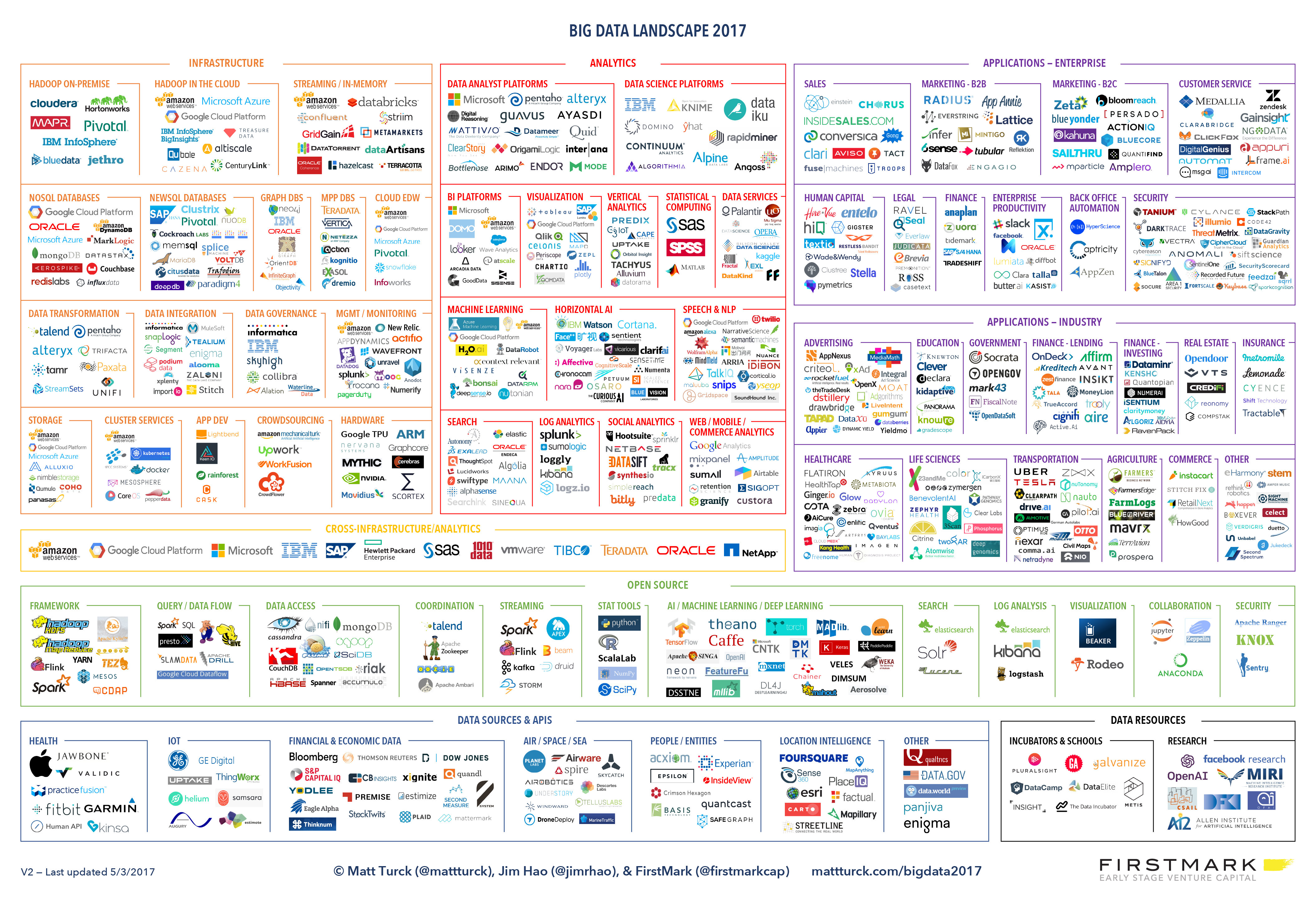
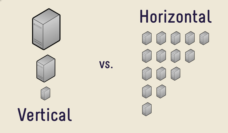